I-LOFAR Observers Guide
- Quickstart Guide
- Acronyms / Jargon / Etc
- Preparing Observation Schedules
- Preparing Observation Schedules With `prepquick.py`
- Queuing an Observation Schedule
- Interrupting Scheduled Observations
- Processing Pulsar Data
- Processing Solar Data (Basic)
- Processing Other Data (EMPTY)
- Bash Aliases
- Station Data Products
- Observing with the Station (LCU)
- Software Levels
- Observing Bit Mode
- Antenna Sets, Subbands and RCU Bands (Modes)
- Beamforming the Station
- Example Observations (Currently only HBA)
- Checking Antenna Spectra
- Command References
- Generating XST Data (Empty)
- Mode 357 (Breaking the Station in the Name of Science) (Empty)
- Observing with the Station (REALTA)
- Station Services
- Archived Pages
- (Archived) Handling Combined Solar/KBT/Beamformed Observations
- (Archived) Handling KBT/Solar357 Observations (ScheduleKBT.py Method)
- (Archived) Executing a Schedule and Processing Data
- A Week in the Life of an I-LOFAR Chief Observer
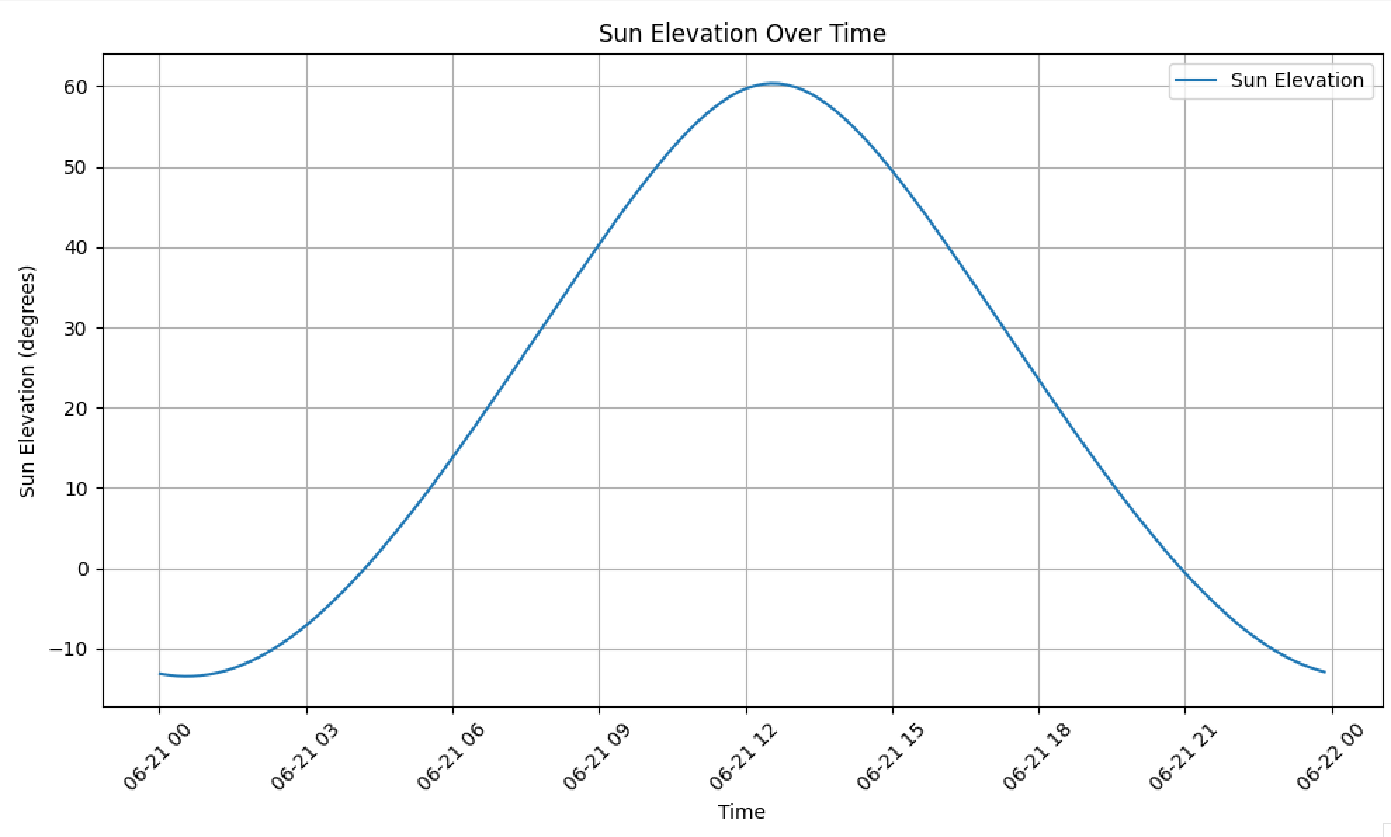
- Scheduling the Sun
Quickstart Guide
Acronyms / Jargon / Etc
Machines
LGC - Linux gateway computer, main node used to access the LCU and REALTA
LCU - Linux control unit, the telescope's brain, used to configure observations, accessibly only via the LGC on the ilofar user
ucc1 - Main recording machine
Paths
REALTA:/mnt/ucc1_recording2/data/observations/YYYY_MM_DD - recording drive path
REALTA:/mnt/ucc1_recording2/data/scripts - recording scripts locations
ilofar@LGC:~/scheduling/schedules - input schedule file folder
Concepts
Software level (swlevel)
- 0 - Station is shutdown
- 1 - Station has basic power
- 2 - Minimum observing mode, hardware can generate antenna correlations
- 3 - Station is fully setup and can beam-form
- 4+ are not needed in a quick-start guide
RCU Modes
- 3: LBA, 0 - 100MHz
- 5: HBAlo, 100 - 200MHz
- 7: HBAhi, 200 - 250MHz
Data products
- BST: typically 1 second cadence data
- XST: Antenna cross-correlations for all-sky imaging
- CEP/REALTA Data: The 3Gbps data stream containing 5.12us data
Preparing Observation Schedules
Scheduling Observations
Observations are typically scheduled using scripts that execute the quicksched.py script found on the LGC. This is a python3.6+ script that takes in a file with schedule entries in a specified format, and then produces two files to observe the specified sources with the HBAs in mode 5 from subbands 12 to 499.
The telescope typically takes 3 minutes in order to be configured before the first (and any STOPSTART) observation begins to produce real data. Additionally it is not uncommon for station handover to occur late. Ensure you consider these points when scheduling high priority observations.
Each entry roughly follows the format
YYYY-MM-DDTHH:MM - YYYY-MM-DDTHH:MM :<TAB>SourceName [RightAscentionRadians, DeclinationRadians, 'COORDINATEBASIS']These can be chained together to form a schedule that looks like this.
2021-09-20T19:30 - 2021-09-20T20:29 :	J1931+4229 [5.110297162889553, 5.110297162889553, 'J2000']
2021-09-20T20:30 - 2021-09-20T20:49 :	B1951+32_PSR [5.20531221260202, 0.5738302241353217, 'J2000']
After running python3 quicksched.py --no-write my_schedule.txt, it will notify you of any issues with the input, or give you a summary of the observations taking place.
Entry Modifiers
STOPSTART: In the case that other observations are scheduled using other software, and you need to leave a gap, you can add STOPSTART to the end of the line after the gap takes place. Whenever this keyword is detected, the station shuts down after the previous observation, then starts up 3 minutes before the given scheduled observation is meant to begin. As an example, these observations will run from 19:27 - 20:29, bring the station down to swlevel 0 for an hour, bring the station up at 21:30, and finally run again from 21:33 - 21:59 before returning the station to software level 0.
2021-09-20T19:30 - 2021-09-20T19:59 :	J1931+4229 [5.110297162889553, 5.110297162889553, 'J2000']
2021-09-20T20:00 - 2021-09-20T20:29 :	B1951+32_PSR [5.20531221260202, 0.5738302241353217, 'J2000']
2021-09-20T21:33 - 2021-09-20T21:59 : J1931+4229 [5.110297162889553, 5.110297162889553, 'J2000'] STOPSTART[IGNORE_ELEVATION]: In the case that a source will be below the default minimum elevation (typically between 10 and 15 degrees depending on setup), the quicksched.py script will reject the observation. If you intend to observe the source at such a low elevation, you can include [IGNORE_ELEVATION] to highlight that you intend to observe this source at a low elevation and the script will proceed without highlighting the elevation of the source.
2021-09-20T19:30 - 2021-09-20T19:59 :	J1931+4229 [5.110297162889553, 5.110297162889553, 'J2000']
2021-09-20T21:33 - 2021-09-20T21:59 : J1931+4229 [5.110297162889553, 5.110297162889553, 'J2000'] [IGNORE_ELEVATION][MODEN]: Where N is replaced with an observing mode (3-7), this will change the observing antenna and frequencies from the mode 5 default to the specified mode as needed.
Further validation is needed for mode 6, as it sometimes fails to change the clock mode.
2021-09-20T19:30 - 2021-09-20T19:59 :	J1931+4229 [5.110297162889553, 5.110297162889553, 'J2000'] [MODE3] # LBA Obs
2021-09-20T20:00 - 2021-09-20T20:29 :	J1931+4229 [5.110297162889553, 5.110297162889553, 'J2000'] # HBALo Obs
2021-09-20T20:30 - 2021-09-20T20:59 : J1931+4229 [5.110297162889553, 5.110297162889553, 'J2000'] [MODE7] # HBAhi obsOR(TOGGLE_FILE): Where "TOGGLE_FILE" is replaced with a file name of choice, this modifier can be used to switch between two observations during schedule execution based on the existence of a file. By default, the first entry on a line will be performed if the file does not exist, while the second will be executed if it does exist. Two files need to be created to perform a toggle: one in the observation folder, and another in the recording folder. Typically, the file name is prefixed by "NOT_" to make it clear that it is disabling the first observation, and enabling the second.
The file must be created before the end of the last observation, otherwise the default observation will be performed.
For I-LOFAR observers, there is a toggle_obs.sh script that will create the input filename in the correct directories for you.
After an observation is switched, the file is removed. As a result, it is not recommended to use the same file name for multiple switches, unless the observer wants to re-create the same file multiple times.
2022-07-19T17:00 - 2022-07-19T17:59 :	FRB20200120E [2.6090272489593733, 1.2012325539587194, 'J2000'] OR(NOT_M81) [Sun357]
2022-07-19T18:00 - 2022-07-19T18:59 :	[Sun357] OR(NOT_SUN) J0939+45 [2.528618475878951, 0.7897614865274342, 'J2000']
Preparing Observation Schedules With `prepquick.py`
The `prepquick.py` script can be used to generate a number of candidate observation windows, based on transit time and observation length, or on source elevation. Each file must start with a start time, which can then be followed by a number of lines with source names, coordinates and information regarding the observation length.
Any information on a line after a '#' is not parsed.
The script does not attempt to realign overlapping observations, you must manually fix these issues before quicksched.py will accept them.
Defining Sources
Sources can be defined by either a set of coordinates in a common basis (J2000, SUN, JUPITER, etc.) or by a name recognised by the CDS, which will be queried by an astropy.coordinates.SkyCoord.from_name() call.
Most solar entries will be automatically converted to mode 357 entries.
Here's an example set of inputs and outputs in both forms, with the time specifiers removed for clarity:
#input.txt
Sun
Moon
PSR B1951+32
J0054+66 [0.23561944901923448, 1.1664616585719019, 'J2000']
TVLM 513-46

#output.txt (self rearranged by start time)
[Sun357]
J0054+66_PSR [0.23561944901923448, 1.1664616585719019, 'J2000']
MOON [0, 0, 'MOON']
TVLM_513-46 [3.931949476576734, 0.3985272105537257, 'J2000']
B1951+32_PSR [5.205312212078421, 0.5738302241353217, 'J2000']
Observing by Elevation
You can get the observing window for a source while it is above a certain elevation by appending a tilde and elevation in degrees. The elevation will be overruled by the value of the `--cutoff` flag if it is set too low.
# input.txt
2023-04-05T00:00:00.000
Sun ~ 15
J0139+3336 ~ 45
Jupiter ~ 20

# output.txt
2023-04-05T07:40 - 2023-04-05T17:24 :	[Sun357]
2023-04-05T08:30 - 2023-04-05T17:14 :	JUPITER [0, 0, 'JUPITER']
2023-04-05T09:25 - 2023-04-05T17:09 :	J0139+3336_PSR [0.4361308670963172, 0.586720056619953, 'J2000']
Observing by Observation Lengths
Otherwise, you can use an observation length to get a candidate schedule for a source by appending a tilde and an observation window in minutes. Note that due to the necessary time needed between beam switches, a minute will be subtracted from this time.
# input.txt
2023-04-05T00:00
Sun @ 75
J0139+3336 @ 120
Jupiter @ 30

# output.txt
2023-04-05T12:00 - 2023-04-05T13:14 :	[Sun357]
2023-04-05T12:20 - 2023-04-05T14:19 :	J0139+3336_PSR [0.4361308670963172, 0.586720056619953, 'J2000']
2023-04-05T12:40 - 2023-04-05T13:09 :	JUPITER [0, 0, 'JUPITER']
Times
A starting line containing a ISOT-formatted date/time string is required in order to determine the source transits. One or more of these lines can be included in the file, and all following sources will be parsed using the last provided timestamp.
The script will determine the next transit after a given time (be it in 5 minutes or 23 hours), and produce the scheduling line candidate based on that. Here is an example that combines each of the described properties above, alongside using multiple different transit times.
# input.txt
2023-05-30T06:00
Sun ~ 15
Moon @ 20
PSR B1951+32 @ 20
J0054+66 [0.23561944901923448, 1.1664616585719019, 'J2000'] @ 20
TVLM 513-46 ~ 55

# New day, new observations
2023-06-01T18:00:00.000
Sun ~ 45
J0139+3336 ~ 45
Jupiter ~ 20

2023-06-03T11:00:00.000
Sun ~ 45


# output.txt
2023-05-30T06:10 - 2023-05-30T18:44 :	[Sun357]
# Note the overlap of this observation, this needs manual tweaking
2023-05-30T08:45 - 2023-05-30T09:04 :	J0054+66_PSR [0.23561944901923448, 1.1664616585719019, 'J2000']
2023-05-30T20:15 - 2023-05-30T20:34 :	MOON [0, 0, 'MOON']
2023-05-30T21:25 - 2023-05-31T00:29 :	TVLM_513-46 [3.931949476576734, 0.3985272105537257, 'J2000']

2023-05-31T03:40 - 2023-05-31T03:59 :	B1951+32_PSR [5.205312212078421, 0.5738302241353217, 'J2000']

2023-06-02T05:05 - 2023-06-02T14:39 :	JUPITER [0, 0, 'JUPITER']
2023-06-02T05:35 - 2023-06-02T13:19 :	J0139+3336_PSR [0.4361308670963172, 0.586720056619953, 'J2000']
# Note that this sun entry is the day after the time stamp provided
2023-06-02T09:35 - 2023-06-02T15:19 :	[Sun357]

2023-06-03T09:35 - 2023-06-03T15:19 : [Sun357]Queuing an Observation Schedule
Working in the scheduling directory is strongly discouraged. It will very likely lead to frustration and spam for any other users on the ilofar account. It is advised to prepare schedules on your local machine or in the temp folder.
Once you have used the previous two guides to build a schedule file, you can then send it to be queued for observations. The schedule should be moved into directory at /home/ilofar/scheduling/schedules by whatever is determined the preferred method. On the ilofar user, the folder can be quickly accessed using the sched alias.
Once the file is in the folder, the monitoring service should notify you and pick up the file. It will be validated with the quicksched.py script, and then either moved to one of the prepared or failed directories, depending on the output. In the case of failure, the logs should be piped to you, or they will be accessible in the logs folder inside the scheduling directory. The file can be modified in the failed directory, and moved back one directory once you believe the issue is resolved.
A second monitoring process check for any files in the prepared directory initially when the files are moved in to the directory, then every 4 hours afterwards. If a schedule starts within the next 24 hours, it will be queued for execution, after which the interrupt.sh script will be needed to exit the opened shells, screens and tmux's before submitting a replacement schedule.
dmckenna@americano:~/git/scheduling$ rsync -avhP ./sched_2023-06-06.txt ~/scheduling/schedules/tmp/sched_2023-06-06.txt
dmckenna@americano:~/git/scheduling$ ssh ilofar@lgc

ilofar@LGC:~$ sched
ilofar@LGC:~/scheduling/schedules$ cat ./tmp/sched_2023-06-06.txt
2023-06-06T07:00 - 2023-06-06T13:29 :	[Sun357]
2023-06-06T13:30 - 2023-06-06T13:59 :	Crab_PSR [1.4596732110242794, 0.3842252837309499, 'J2000']
ilofar@LGC:~/scheduling/schedules$ mv ./tmp/sched_2023-06-06.txt ./
ilofar@LGC:~/scheduling/schedules$
Message from ilofar@LGC on (none) at 15:16 ...
Attempting to parse new input schedule at /home/ilofar/scheduling/schedules/sched_2023-06-06.txt
EOF

Message from ilofar@LGC on (none) at 15:16 ...
/home/ilofar/scheduling/schedules/sched_2023-06-06.txt: Success; moving schedule to the /home/ilofar/scheduling/schedules/prepared/ directory.
EOF
<ENTER>
ilofar@LGC:~/scheduling/schedules$ Interrupting Scheduled Observations
The interruptObs.sh script operates in one of two modes: focused and global. In focused mode, it will take an input schedule, determine the relevant launched instances for that schedule, and specifically shut down all related screens, tmuxes and processes. In global mode, the script will kill anything related to our scheduling scripts.
See date(1) (-d input) for further details on accepted time stamps. We also support "next" in focused mode, which will parse the input file, find the next gap between observations, and perform the switch then to minimise downtime.
Focused Mode
In focused mode, you must provide at least an interruption time (in a format accepted by date), and a reference schedule to analyse. You can optionally provide a third parameter with a replacement schedule if you do not want to manually staged and run another schedule afterwards. These are all valid examples for killing a specified "./schedule/my_sched.txt" schedule file.
ilofar@LGC:~/workdir$ interruptObs.sh 2023-06-01T07:00:00 ./myschedule.txt
ilofar@LGC:~/workdir$ interruptObs.sh now ./myschedule.txt
ilofar@LGC:~/workdir$ interruptObs.sh now ~/scheduling/schedules/staged/sched_2023-06-01.txt
ilofar@LGC:~/workdir$ interruptObs.sh next ~/scheduling/schedules/staged/sched_2023-06-01.txt schedule_replacement.txt
Global Mode
In global mode, you just need to specify a time and the "KILLALL" keyword as the schedule. After this, it will find any running scripts, screens, tmuxes, etc, on both the recording node, LCU, and local node that are associated with scheduling and kill them. This should typically only be used in the case that something has gone horribly wrong.
ilofar@LGC:~/workdir$ interruptObs.sh 2023-06-01T07:00:00 KILLALL
ilofar@LGC:~/workdir$ interruptObs.sh now KILLALLProcessing Pulsar Data
CDMT (Stokes I) Method
The GPUs in ucc4 are typically used to reduce the majority of the pulsar data produced by the station into mode 5, 8x channelised, 16x downsampled Sigproc Stokes I filterbanks. This is achieved through using a python3 script, cdmtProc.py, to produce a bash script with the correct flags needed to call CDMT with maximum performance, while not overutilising the GPU's VRAM.
The script needs to be provided a path to the recording folder, and optionally an extension to add to the file name. The resulting bash script can then be executed. Once data is analysed, the compress.sh and transfer.sh scripts can be used to compress the raw data using zstandard, then transfer it to the DIAS archive.
obs@ucc4:~$ tmux new
obs@ucc4:~$ dckrgpu

root@b02cf5b93fbc:/home/user# cd /mnt/ucc4_data2/data/David/
root@b02cf5b93fbc:/mnt/ucc4_data2/data/David# mkdir rrat_2023_05_30
root@b02cf5b93fbc:/mnt/ucc4_data2/data/David# cd rrat_2023_05_30
root@b02cf5b93fbc:/mnt/ucc4_data2/data/David/rrat_2023_05_30# cp ../cdmtProc.py ./
root@b02cf5b93fbc:/mnt/ucc4_data2/data/David/rrat_2023_05_30# python3 cdmtProc.py -i /mnt/ucc1_recording2/data/rrats/2023_05_30/ --extra 1
root@b02cf5b93fbc:/mnt/ucc4_data2/data/David/rrat_2023_05_30# ll
total 92
drwxr-xr-x   2 root root  4096 May 30 15:48 ./
drwxr-xr-x 129 1000 1000 69632 May 30 15:47 ../
-rw-r--r--   1 root root 14501 May 30 15:47 cdmtProc.py
-rw-r--r--   1 root root   886 May 30 15:48 cdmtProc_1.sh
root@b02cf5b93fbc:/mnt/ucc4_data2/data/David/rrat_2023_05_30# bash cdmtProc_1.sh

<data is processed>

root@b02cf5b93fbc:/mnt/ucc4_data2/data/David/rrat_2023_05_30# bash ../compress.sh; bash ../transfer.sh
Single Pulse, Periodic Emission Searches
Two scripts in the /mnt/ucc4_data2/data/David/ directory can be used to setup single pulse searches.
The generateHeimdall.py script will open a number of matplotlib interfaces with bandpasses for RFI flagging before writing a list of narrow and wide DM searches for single pulses data. When flagging the data, each click on the bandpass will flag a subband worth of data (8 channels), and a range of subbands can be flagged by clicking somewhere, moving the mouse to the end of the range, then pressing "a" with the window active. The output script will be in the cands/ subdirectory of the input folder.
The candidate files are then used to generate plots of each pulse that fits certain criteria (typically SNR > 7.5, width < 2**10 samples). This process is automated with the frb_v4.py and generateCands.py scripts.
dmckenna@ucc2:/mnt/ucc2_data1/data/dmckenna/working_cands$ mkdir rrat_2023_05_30
dmckenna@ucc2:/mnt/ucc2_data1/data/dmckenna/working_cands$ cd rrat_2023_05_30
dmckenna@ucc2:/mnt/ucc2_data1/data/dmckenna/working_cands/rrat_2023_05_30$ cp ../frb_v4.py .
dmckenna@ucc2:/mnt/ucc2_data1/data/dmckenna/working_cands/rrat_2023_05_30$ for i in {1..4}; do python3.8 ../generateCands.py -i /mnt/ucc4_data2/data/David/rrat_2023_05_30/ -o proc_ucc4_${i}.sh; bash proc_ucc4_${i}.sh; sleep 3600; done
The generatePrepfolds.py script will generate a list of rfifind and prepfold commands for both set targets, and targets within 1 degree of the original pointing. The output script will be in the folds/ subdirectory of the input folder.
Single pulse candidates and folded profiles can then be copied locally, with folded profiles converted from ps files to png using the grabFolds.sh script.
udpPacketManager/digifil (Stokes IQUV) Method
For full Stokes IQUV data, we use udpPacketManager to convert the raw CEP data into a DADA data block, which is then processed with digifil. The script for automating this need to be modified to contain a dispersion measure for coherent dedispersion, and a downsampling fact for the data. Afterwards, the script can be run, pointed at a specific directory, and it will handle the rest for you.
obs@ucc1:~$ tmux new
obs@ucc1:~$ bash /mnt/ucc1_recording2/data/rrats/4pol/enter_docker.sh

root@106316e58e36:/home/user# cd /mnt/ucc1_recording2/data/rrats/2023_05_30/
root@106316e58e36:/mnt/ucc1_recording2/data/rrats/2023_05_30# mkdir tmp_processing
root@106316e58e36:/mnt/ucc1_recording2/data/rrats/2023_05_30# cd tmp_processing
root@106316e58e36:/mnt/ucc1_recording2/data/rrats/2023_05_30/tmp_processing# cp ../../4pol/* ./
root@106316e58e36:/mnt/ucc1_recording2/data/rrats/2023_05_30/tmp_processing# bash 4pol_generate.sh

# Alternatively,
root@106316e58e36:/home/user# cd /mnt/ucc1_recording2/data/rrats/prcoessing/
root@106316e58e36:/mnt/ucc1_recording2/data/rrats/processing# mkdir 2023_05_30
root@106316e58e36:/mnt/ucc1_recording2/data/rrats/processing# cd 2023_05_30
root@106316e58e36:/mnt/ucc1_recording2/data/rrats/processing/2023_05_30# cp ../../4pol/* ./
root@106316e58e36:/mnt/ucc1_recording2/data/rrats/processing/2023_05_30# bash 4pol_generate.sh /mnt/ucc1_recording2/data/rrats/2023_05_30/Processing Solar Data (Basic)
UPM Method
Solar data is typically processed using udpPacketManager, to produce a Stokes IV output, downsampled by a factor of 256 to 1.3ms, using a set of automated scripts.
The process_data.sh script can be set to process any subdirectories with data on a specific path, or will automatically find the newest directory of observations, and process any Solar observations.
The series of commands needed to setup a processing run can be found in the code block below.
obs@ucc1:~$ cdrs
obs@ucc1:/mnt/ucc1_recording2/data/sun$ mkdir 20230530_sun357
obs@ucc1:/mnt/ucc1_recording2/data/sun$ cd 20230530_sun357
obs@ucc1:/mnt/ucc1_recording2/data/sun/20230530_sun357$ cp ../templates/* ./
obs@ucc1:/mnt/ucc1_recording2/data/sun/20230530_sun357$ bash enter_docker.sh

root@2639bfd271d6:/home/user# cd $LAST_DIR
root@2639bfd271d6:/mnt/ucc1_recording2/data/sun/20230530_sun357# bash process_data.sh

# Alternatively
root@2639bfd271d6:/home/user# cd $LAST_DIR
root@2639bfd271d6:/mnt/ucc1_recording2/data/sun/20230530_sun357# bash process_data.sh /mnt/ucc1_recording2/data/rrats/2023_05_30/

# After processing
root@2639bfd271d6:/mnt/ucc1_recording2/data/sun/20230530_sun357# exit
obs@ucc1:/mnt/ucc1_recording2/data/sun/20230530_sun357$ bash transfer.shProcessing Other Data (EMPTY)
UPM Method
Bash Aliases
LGC
$ # Access the LCU while in local mode
$ lcu

$ # Access the Recording node (ucc1)
$ ucc1

$ # Access the scheduling directory
$ sched

$ # Test a schedule file
$ testsched my_input_file.txt
UCC1
$ # Access recording drive 1 (old)
$ cdr
$ # Access the active recording drive
$ cdr2

$ # View the remaining storage on the recording drives
$ dfr

$ # See the disk usage of the current subdirectories
$ duds

$ # Access the recorded observations directory
$ cdo
$ # Access the last recorded observation
$ cdol

$ # Access the RRATs processing directory (old recording directory)
$ cdrr
$ # Access the latest RRAT directory
$ cdrrl

$ # Access the Solar processing directory
$ cdrs
$ # Access the latest Solar directory
$ cdrsl
Station Data Products
An overall description of the output products of an international LOFAR station, and pointing out the small details that are left out of the cookbook.
Introduction
Most of the information in this chapter can be found within the LOFAR Station Cookbook, though there are a few other handy additions regarding the output formats that can be of interest. We will also discuss the current methogology for handling the data products and converting them to other formats, if needed.
XST Data
Array correlation/crosslet statistics statistics (XSTs) describe the autocorrelation between different antenna for a single subband at a given point in time (visibilities, covariances). A single XST file contains a single subband's data, which differs from a ACC file which loops over a range of subbands. They can be used to generate all-sky maps, a representation of the sky birghtness distribution of the station at a given frequency.
Generating XSTs
XSTs are generated using the rspctl command while the station is in swlevel 2 , a known mode is set by rspctl --mode=N or rspctl --band=N_M and the station is expected to be in bitmode 16 as no other observations can be performed simultaneously. It will generate an output intergrated over the last Nsec to a file in a given local_folder . The overall syntax to generate an output for a given subband is
user1@lcu$ rspctl --xcsubband=subband
user1@lcu$ rspctl --xcstatistics --duration=n_observation_seconds --integration=n_sec --directory=local_folder
It is recommended to run this in combination with a script that will move the file to a new location after Nobservation_sec as the file contains no metadata of the mode or subband used for the observation. Moving to a specified modeN/sbM/ subband is highly recommend as a result. A sample observing script, assuming the station is in swlevel 2 can be found here.
A note on HBA all-sky observations
Due to the rigid tile structure of the HBAs aligning the side lobes, performing all-sky observations with the entire HBA array is a hopeless endeavour.
However, at the GLOW stations, James Anderson worked around this by activating a single antenna in each HBA tile in a pesudo-random fashion to minimise sidelobe collision. Further work on the methodology by Menno Norden and Michiel Brentjens optimized this method and resulted in the script found here, slightly modified for use on the Irish station, which will automate the process for you. It should be run before any attempts to perform all-sky observations with the HBA tiles.
XST Data Format
XSTs are antenna-majour files that are written to disk every integration period. They do not come with any metadata outside of the starting time, which is present in the file name.
Each sample is 4 x Nantenna x Nantenna long (by default, an international station has 96 antenna). Each antenna generates a real and imaginary sample for it's correlation with every other antenna (Complex128 type, 2 Float64s, for each polarization). As a result, at the (n,n) indictes we generate the autocorrelation of the antenna with no lag. The overall format can be thought of as a 3D cube, with (n,n) squares stacked for m time samples.
| (N0,N0) | (N0,N1) | ... | (N0,Nn) |
| (N1,N0) | (N1,N1) | ||
| ... | ... | ||
| (Nn,N0) | (Nn,Nn) |
All-Sky Plotting
Some sample mode 3, subband 210 data from IE613 can be found here. it is highly recommended to use an existing implementation for generating all-sky images, I provide the example David worked on here, but there is also Griffin Foster's SWHT, a module inside Tobia Carozzi's iLiSA and some scripts floating around the LOFAR community.
The method for generating all-sky maps is heavily involed and as a result we will only outline the steps involved here.
- Acquire XST data, antenna locations and (optionally) calibrations files for your station
- Load your data and metadata into an eniroment, samples for XST and calibrtion data,
xstData = np.fromfile(dataRef, dtype = np.complex128)
reshapeSize = xstData.size / (192 ** 2)
xstData = xstData.reshape(192, 192, reshapeSize, order = 'F')

calData = np.fromfile(calRef, dtype = np.complex128)
rcuCount = calVar.size / 512
calData = calData.reshape(rcuCount, 512, order = 'F')
calData = calData[:, subband_of_interest]

calXData = calData[::2]
calYData = calData[1::2]
calData = np.dstack([calXData, calYData])- Apply your calibrations if needed to each of the X/Y polarizations
calSubbandX = calData[:, subband, 0]
calSubbandY = calData[:, subband, 1]

calMatrixXArr = np.outer(calSubbandX, np.conj(calSubbandX).T)[..., np.newaxis]
inputCorrelations[::2, ::2, ...] = np.multiply(np.conj(calMatrixXArr), inputCorrelations[::2, ::2, ...])

calMatrixYArr = np.outer(calSubbandY, np.conj(calSubbandY).T)[..., np.newaxis]
inputCorrelations[1::2, 1::2, ...] = np.multiply(np.conj(calMatrixYArr), inputCorrelations[1::2, 1::2, ...])- Generate a range of pointings from sin(-pi/2) -> sin(+pi/2) across a grid, lower values will limit your field of view ((l,m) grid size)
- Calculate your wavelength and corresponding wavenumber for your subband (
k = (2 * np.pi) / wavelength) - Form a weight matrix (and it's conjugate) for your pointing using the x-coordinates and y-coordinates of your antennae
wX = np.exp(-1j * k * posX * lVec) # (l, 96)
wY = np.exp(-1j * k * posY * mVec) # (m, 96)
weight = np.multiply(wX[:, np.newaxis, :], wY[:, :, np.newaxis]).transpose((1,2,0))[..., np.newaxis] # (l,m,96,1)
conjWeight = np.conj(weight).transpose((0,1,3,2)) # (l,m,1,96)- For each sample of correlations, find the dot product of the correations with the complex conjugate of your weight matrix, and then the weight matrix
for frame in np.arange(frameCount):
	correlationMatrixChan = correlationMatrix[..., frame] # (96,96)
	tempProd = np.dot(conjWeight, correlationMatrixChan) # w.H * corr # (l,m, 1, 96)
	prodProd = np.multiply(tempProd.transpose((0,1,3,2)), weight)
	outputFrame[..., frame] = np.sum(prodProd, axis = (2,3))
Your output image will need to be rotated by the same mount as your station is rotated. You can find that information within the new iHBADeltas.conf files.
BST Data
Beamlet statictics (BSTs) are effectively dyanmic spectra produced by the station at a regular, relatively low cadence, interval.
Generating BSTs
BSTs are generated using the rspctl command in conjunction with a running beamctl command (as a result, the station must be in at least swlevel 3). It will write an output summary of the last Nsec (int) of antenna correlations to disk in a given folder_location. The overall synctax to call a rspctl command is
user1@lcu$ rspctl --statistics=beamlet --duration=n_observation_sec --integration=n_sec --directory=folder_location/The rspctl command will generate data for Nobservation_sec or until the process is killed. As a result, the process must be kept active in a screen or by trailing the execution with an ampersand to send it to the background.
Enabling BST generation with the rspctl command will disable the CEP packet data stream, which can be re-enabled afterwards by calling $ rspctl --datastream=1 . You can verify this worked by calling $ rspctl --datastream to get the current status of the datastream.
BST Data Format
BSTs are frequency-majour files that are written to disk every integration period. They do not come with any metadata outside of the stating time, output ring (only 0 available to international stations) and antenna polarization which are visible within the file name.
Each beamlet controlled by a beamctl command will generate a single output sample per intergration. So the output array dimensions will depend on your observation, and may be up to 244 in 16-bit mode, 488 in 8-bit mode and 976 in 4-bit mode.
The output data is a float, 4 times the size of your input.
| Bitmode | Output (float) |
| 4 | float32 (verify) |
| 8 | float64 |
| 16 | float128 |
BST Plotting
A fast way to plot BSTs in Python can be achieved with the numpy and matplotlib libraries. If you want to test this out for yourself, there are a large number of BSTs available on the data.lofar.ie archive which contain 488 subband observations from our Solar monitoring campaign.
import numpy as np
import matplotlib.pyplot as plt

bstLocation = "/path/to/bst.dat"
#bstDtype = np.float32 # 4-bit obs
#bstDtype = np.float64 # 8-bit obs
#bstDtype = np.float128 # 16-bit obs
rawData = np.fromfile(bstLocation, dtype = bstDtype)

#numBeamlets = 976 # 4-bit obs
#numBeamlets = 488 # 8-bit obs
#numBeamlets = 244 # 16-bit obs
rawData = rawData.reshape(-1, numBeamlets)


plt.figure(figsize=(24,12))
plt.imshow(np.log10(rawData.T), aspect = "auto")
plt.xlabel("Time Samples"); plt.ylabel("Subband"); plt.title("BST Data ({})".format(bstLocation))
plt.show()ACC Data
Array correlation/crosslet statistics statistics (ACCs) describe the autocorrelation between different antenna for a number of subbands across a period of time (visibilities, covariances). A single ACC file typically contains one or more scans across the entire subband range of an observing mode, which differs from a XST file which only observed a single subband. They can be used to generate all-sky maps, a representation of the sky brightness distribution of the station at a given frequency, though typically ACCs are used for station debugging and calibration
Generating ACCs (Validation Required)
ACCs are generated using the rspctl command while the station is in swlevel 2 , a known mode is set by rspctl --mode=N or rspctl --band=N_M and the station is expected to be in bitmode 16 as no other observations can be performed simultaneously. It will generate an output integrated over the last Nsec to a file in a given local_folder . The overall syntax to generate an output is
user1@lcu$ rspctl --xcstatistics --duration=n_observation_seconds --integration=n_sec --directory=local_folderThis differs from XSTs as no subband is specified. It is recommended to keep the observing mode in the local_folder name due to the lack of metadata associated with the observation.
You are also recommended to check in with your observer or station configuration to see the subbands the scan will be performed over. While by default, this covers every subband in a given mode before looking, your configuration may have changed and only use a limited subset of frequency channels.
A note on HBA all-sky observations
Due to the rigid tile structure of the HBAs aligning the side lobes, performing all-sky observations with the entire HBA array is a hopeless endeavour.
However, at the GLOW stations, James Anderson worked around this by activating a single antenna in each HBA tile in a pesudo-random fashion to minimise sidelobe collision. Further work on the methodology by Menno Norden and Michiel Brentjens optimized this method and resulted in the script found here, slightly modified for use on the Irish station, which will automate the process for you. It should be run before any attempts to perform all-sky observations with the HBA tiles.
ACC Data Format (Validation Required)
ACCs are antenna-major files that are written to disk every integration period for each subband. They do not come with any metadata outside of the starting time, which is present in the file name.
Each sample is 4 x Nsubbands x Nantenna x Nantenna long (by default, an international station has 96 antenna). Each antenna generates a real and imaginary sample for it's correlation with every other antenna (Complex128 type, 2 Float64s, for each polarization). As a result, at the (n,n) indictes we generate the autocorrelation of the antenna with no lag. The overall format can be thought of as a 3D cube, with (n,n) squares stacked for m time samples.
| (N0,N0) | (N0,N1) | ... | (N0,Nn) |
| (N1,N0) | (N1,N1) | ||
| ... | ... | ||
| (Nn,N0) | (Nn,Nn) |
Each sample above is the index of 2 Complex128 values, for each polarizations of an antenna pair, giving an overall dimension of (192, 192) Complex128 elements for a standard international station.
See the "XST Data" page for an explanation on using these data products for all-sky maps.
CEP Packet Stream
The CEP packet stream is the lowest level, constantly produced data product from the station. It is a series of UDP packets that provide information on the digitized voltages for a given antenna while a beamformed observaiton is performed. There are normally 4 ports of data produced, though this may be lower if you are not fully utilizing the beamlets available to your station.
The CEP packet stream is highly variable, based on both your observing setup and your RSP configuration (/var/lofar/etc/RSPDriver.conf), we will describe this format as generic as ossible and provide default values for an international station.
Generating the CEP Packet Stream
The CEP packet stream should be generated whenever a beamformed observation is started via beamctl, though your station ocnfiguration or the use of rspctl to create BST data may interrupt or stop the data stream. You can verify the stream is enabled through the rspctl --datastream command, and re-enable it by calling rspctl --datastream=1.
While enabled, the CEP packet stream will send data to the MAC addresses configured in your RSPDRiver.conf every N time samples (by default, 16, 81.92µs) on all ports; though some ports may not contain data if the beamlets are not allocated. The subbands are distributed as described below (values are always inclusive).
| Port Offset | 4-bit Data | 8-bit Data | 16- bit Data |
| 0 | 0:243 | 0:121 | 0:60 |
| 1 | 244:487 | 122:243 | 61:121 |
| 2 | 488:731 | 244:365 | 122:182 |
| 3 | 732:975 | 366:487 | 183:243 |
As the packets are UDP packets, the data may arrive at your machine out of order or not arrive at all. Packet loss to on-site machines is normally relatively low and in-order, so performing operations on the raw recorded data should be fine for more cases.
CEP Packet Data Format
The full CEP packet is described on page 32 of the Station Cookbook, but for now we will focus in on the CEP header, without any of the UDP information, and the raw data
There are 16 bytes of relelvant information at the start of every CEP packet. While it doesn't provide as much metatdata as we wouldl ike, it gives a good starting point for validation the structure of a packet and some of the base observing parameters.
| Parameter | Byte(:bit) | Usage | ||
| RSP Version | 0 | Validation (~=3) | ||
| Source Info | 1-2 | Observing Configuration | ||
| RSP ID | 1:0-4 (5-bit) | Output RSP ID | ||
| Unused | 1:5 (1-bit) | Validate 0 | ||
| RSP Error | 1:6 (1-bit) | RSP Error, validate 0 | ||
| Clock Bit | 1:7 (1-bit) | 1 if 200MHz clock, 0 if 160MHz | ||
| Bit mode | 2:0-1 (2-bit) | 0: 16-bit, 1: 8-bit: 2: 4-bit, 3: ERR | ||
| Unused | 2:2-7 (6-bit) | Vaidate 0 | ||
| Config | 3 | |||
| Station ID | 4-5 | Station Code (see below) | ||
| Number of beamets | 6 | Beamlets in the current packet | ||
| Number of time samples | 7 | Time samples in the current packet (normally 16) | ||
| Timestamp | 8-11 | Unix timestamp of observation | ||
| Sequence | 12-15 | Leading time sample sequence | ||
The actual packet size can vary based on the observing methodology. You can predict the size of each packet, and the raw data deminsions as a result, from the number of beamlets and number of time samples (bytes 6 and 7).
The reported statino code does not correspond to the public station names, I.e. IE613, SE607, etc. The RSPs report the internal station code, multiplied by 32, with an offset depending on the output port. The full list of station codes can be found here. As an example, if we were to analyse the short value produced from IE613, we would expect to see (214 * 32) + (0,1,2,3) depending on the CEP port analysed.
The data is then in time-majour order, where each time sample contains the (Xreal, Ximag, Yreal, Yimag) samples. Size of each sample depends on your bitmode, varying from half a byte (4-bit) to 2 bytes (16-bit). This repeats for Ntime sampels (default is 16), before moving on to the next beamlet.
Recording / Handling Methodology
This is discussed more in-dept within the REALTA user's guide where we describe the methodology used at IE613. The overall view is that the data should be
- Recorded with some UDP packet capturing software -- wireshark, Olaf Wucknitz's volage recorder, etc.
- Data is read back either blindly or checking for missing packets, out of sequence data, headers analyzed, etc
- Voltages can be used to form Stokes vectors to the output data product required
TBB Data (Empty)
SST Data (Empty)
Observing with the Station (LCU)
The chapter describe the different observation methods when directly interfacing with the station, rather than using any automated scripts.
The order in which topics are disccused also reflects the order in which commands need to be called to correctly configure the station for an observation.
Software Levels
In international mode, the station has 4 software levels, but only 3 of which are used extensively. Levels are applied consecutively, so entering software level 3 will turn on any services that are normally turned on by software level 1 and 2.
Software level is described and configured with the swlevel command. The two main forms of the command you will use are swlevel <level> and swlevel -S. Examples of this command are given below.
user1@lcu$ # Get the current software level
user1@lcu$ swlevel -S
0
user1@lcu$ # Go to software level 2 for all-sky imaging or antenna statistics collection
user1@lcu$ swlevel 2
<start-up messages>
user1@lcu$ # Go to software level 3 for beamformed observations
user1@lcu$ swlevel 3
<start-up messages>
In some cases, there may be an error during startup, or a service may crash during an observation. If a critical service has been effected, the station will change the software level to be in n invalid state, normally represented by your intended software level multiplied by -1. So if you were in software level 3 and an error occurred, the swlevel -S command will describe the station as being in level -3. To resolve this issue, you can either go to level 0 and back to your target level, or attempt to re-initialise the target level. Often, going to level 0 and back is the safest option and will resolve more issues, though at the cost of time.
At I-LOFAR, a cycle from level 0 to level 3 typically takes between 2 and 3 minutes. Consider this delay when planning your observations.
Software Level 0 (Off)
Software level 0 is the default mode the station is in after handover, and should be returned to before hand-over. In this state, all of the RSP, beaforming and calibration services are stopped and the station is inactive. Between observations the station is sometimes returned to software level 0 to ensure there are no rogue beams, statistic collectors, etc, still running from a previous observation so that the station can be brought up in a fresh state for the next observer.
Software Level 1 (Station Monitoring)
Software level 1 initialises some low-level daemons and the station monitoring and control software. Observations cannot be performed in this mode.
Software Level 2 (Hardware Initialised)
Software level 2 loads images onto the RSPs, enables the RCUs and performs some other low-level operations to prepare the station. While correlation statistic observations should be taken in this mode (XST, ACC), no beamformed observations can be performed in this mode.
Software Level 3 (Software Initialised)
Software level 3 starts the beamforming and calibration services. This is the default mode the station should be in while performing any beamformed observations (any non-XST/ACC observations, though attempting to take these will generate output files, but the correlations may be applied to post-beamforming delayed voltages).
Observing Bit Mode
There are 3 available bit modes available while observing with the station. 4, 8 and 16-bit, each of which describe the size of the signed word of each beamlet sample. 8-bit is the standard mode used for observations with I-LOFAR.
Adjusting the bit mode of the station varies the number of beamlets (pointings, frequencies) that can be formed at a given time, allowing for a trade off between digitisation accuracy and observing bandwidth.
| Bitmode | Beamlets | Bandwidth (MHz) |
| 16 | 244 | 47.65625 |
| 8 | 488 | 95.3125 |
| 4 | 976 | 190.625 |
The bitmode can be set using the rspctl command and the --bitmode flag, as demonstrated below.
user1@lcu$ rspctl --bitmode=16
user1@lcu$ rspctl --bitmode=8
user1@lcu$ rspctl --bitmode=4
4-bit Mode
4-bit mode is rarely used as unlike 8-bit mode, during the reduction operation from 8-bit to 4-bit data is not fully reduced to fit in the -8,7 range, resulting in samples being clipped. This can be compensated for by increasing the RCU attenuation, but requires analysis on a source-by-source basis due to the highly variable sky temperature at low frequencies. Data produced in this mode needs to be extracted in a special way, as each sample takes up the upper or lower half of a single byte.
When used correctly, it can allow for an extremely large sky coverage, or observations across multiple observing modes, at the cost of some sensitivity.
8-bit Mode
8-bit mode is the standard for all HBA and most LBA observations at I-LOFAR, offering up a 95MHz bandwidth for observers to cover an entire observing mode with the 200MHz clock (excluding parts of the Nyquist zones at multiples of 100MHz or 80MHz, depending on your clock mode).
16-bit Mode
16-bit mode is sometimes used for LBA observations to slightly increase the sensitivity at lower frequencies. This is often a useful trade-off due to the significant amount of RFI present below 30MHz from ionospheric reflections and local sources (AM radio, FM radio about 80MHz, etc, making sizeable fractions of the bandwidth unusable).
Antenna Sets, Subbands and RCU Bands (Modes)
Antenna Sets
In international mode, we recommend using either the LBA_OUTER or HBA_JOINED antenna sets, depending on the part of the instrument you intend to use. The remaining antenna sets are mostly used in the core and remote stations depending on the needs of observers to full out different parts of the UV-plane when observing with multiple stations
LBA_OUTER can be used with bands 10_90 or 30_90, while HBA_JOINED can be used with 110_190, 170_230, 210_250. The properties of each of these bands are described below.
The choice of antenna-set and band in your beamctl command, with the --antennaset and --band flags will chose how the station operates.
| RCU Band | RCU Clock (MHz) | Lower Frequency (MHz) | Upper Frequency (MHz) | Subband Width (MHz) |
| 10_90 | 200 | 0 | 100 | 0.1953125 |
| 30_90 | 200 | 0 | 100 | 0.1953125 |
| 110_190 | 200 | 100 | 200 | 0.1953125 |
| 170_230 | 160 | 160 | 240 | 0.15625 |
| 210_250 | 200 | 200 | 300 (~260 effective) | 0.1953125 |
RCU Bands (Modes)
The RCU band (formally known as RCU mode, now referred to as 'bands', configured via the --band flag) allows you to set the observing window for a given set of RCUs. While the band of each antenna polarisation can be configured to be independent on any other antenna (allowing for configurations such as KAIRA's Mode 3-5-7), we recommend only using a single observing band and use multiple observing epochs to see a source over multiple modes to allow for the use of the entire antenna set to maximise the sensitivity and keep a reasonable and predictable beam shape for each observation.
The name of each band roughly describes the frequencies at which the electronics will have a negligible effect on the observed data. Outside of these ranges, the Nyquist zone or other filters may suppress emission at certain frequencies, even if they are available at specific subbands.
Mode 0, 1, 2
These modes are the OFF, Low-band Low (200MHz) and Low-Band Low (160MHz) observation modes, they should not be be used on international stations and are meant to selectively use different parts of the array in the core and remote stations.
Mode 3 (Band '10_90')
Mode 3 is the standard LBA observing mode, using the entire set of LBA antenna and the 200MHz clock, covering 0MHz to 100MHz.
Mode 4 (Band '30_90')
Mode 4 enables observation with the entire set of LBA antenna and the 200MHz clock, with an additional high-pass filter to reduce the effects of bright signals below 30MHz, but allowing for observations from 0MHz to 100MHz.
Mode 5 (Band '110_190', "HBALo")
Mode 5 is the standard HBA observing mode, enables observing with the HBA tiles and the 200MHz clock covering 100MHz to 200MHz.
Mode 6 (Band '170_230')
Mode 6 enables observing with the HBA tiles and the 160MHz clock, covering 160MHz - 240MHz.
Mode 7 (Band '210_250', "HBAHi")
Mode 7 enables observing with the HBA tiles and the 200MHz clock. It has a reduced bandwidth compared to the other modes as a result of significant amounts of RFI and antenna attenuation being present above ~240MHz, but allows for observations from 200MHz to 250MHz.
Subbands
A subband is 1 out of 512 slices created by the polyphase filterbank out of the total bandwidth available to a given observing band. The total bandwidth available is either 100MHz or 80MHz depending on your use of the 200MHz or 160MHz clock (refer to the table above or text below).
When trying to calculate the subbands you are interested in,you will need to consider the frequencies of interest and the chosen observing band. For example, while only 0-100 MHz is available to the LBAs, the HBA can observe either 100-200, 160-240, or 200-260MHz at one point in time. As a result, you should
- Chose your RCU band based on the frequencies of interest, and determine the lowest frequency available to you
- Find the difference between the lowest frequency and your target frequency, and divide the resulting value by the subband width (the RCU clock value divided by 1024), rounded downwards to encapsulate the target frequency, and you have one of your subband limits.
- Repeat for a chosen upper frequency, and ensure that your bitmode allows you to allocate enough beamlets (see previous chapter)
Overall, the subband calculation roughly follows this equation
target_subband = (target_frequency - band_base_frequency) / (band_rcu_clock / 1024)
target_subband = round_down(target_subband)
As some example calculations,
| Frequency (MHz) | Band |
Base Frequency (MHz) |
RSP Clock (MHz) | Sub-band Calculation | Subband |
| 25 | 10_90 | 0 | 200 | (25 - 0) / (200 / 1024) | 128 |
| 125 | 110_190 | 100 | 200 | (125 - 100) / (200 / 1024) | 128 |
| 185 | 170_230 | 160 | 160 | (185 - 160) / (160 / 1024) |
160 |
| 225 | 210_250 | 200 | 200 | (225 - 200) / (200 / 1024) | 128 |
Beamforming the Station
Beamforming is the process by which the station electronics collect the antenna signals and delays the signals to allow them to be coherently summed to point at a certain point in the sky. Depending on your bit-mode, you can control between 244 and 976 of these beams, each of which can take on a unique frequency and pointing direction.
Typically, all beams are pointed in the same direction, with the same antenna-set, and only differ in the selected frequencies. While other pages will discuss why/how we can deviate from that choice, this page will focus on observing a single mode, in bit-mode 8 (to use most of the available bandwidth in a given mode).
General Beamforming
In order to create a beam, you will need to execute a beamctl command. This command will require a spatial configuration, a spectral configuration and an antenna configuration. Roughly, a single beamctl command will look like either of the following stencils. The antenna sets, bands and subband components of these commands have been described elsewhere in this chapter.
user1@lcu$ # Observe with the LBAs
user1@lcu$ beamctl 	--antennaset=LBA_OUTER \
					--rcus=$rcus \
                    --band=$bandLBA  \
                    --beamlets=$beamletsLBA \
                    --subbands=$subbandsLBA \
                    --digdir=$pointing
user1@lcu$
user1@lcu$ # Observe with the HBAs
user1@lcu$ beamctl 	--antennaset=HBA_JOINED \
					--rcus=$rcus \
                    --band=$bandHBA  \
                    --beamlets=$beamletsHBA \
                    --subbands=$subbandsHBA \
                    --anadir=$pointing \
                    --digdir=$pointing
Numeric Lists in LOFAR commands
The inputs to LOFAR commands can contain numeric lists. These lists use both semi-colon indexing to describe a range of inclusive values (e.g., 0:2 represents 0,1,2) and command separated values or lists to refer to multiple separate groups (e.g., 0,1:6,9). Spaces cannot be included in these groups.
When attempting to exclude values, be sure you aren't accidentally including them at the start/end of a range.
RCUs
RCUs represent the LBA antenna or HBA tiles you intend to use for your observations. As of writing, I-LOFAR currently has 1 malfunctioning LBA and 2 malfunctioning HBAs. reaching out to observers will give you the current definitive list of the antenna you should be using for your observations.
When flagging a given antenna or tile, it is recommended to always flag both polarisation to prevent biases from excess intensity in one polarisation than another when beamforming (e.g., you could introduce a +2% bias to Stokes V by only flagging one polarisation).
Beamlets
The allocated beamlets can be anywhere on the range allowed by your chosen software level (e.g., to allocate 200 beamlets in 16-bit mode, I can allocate them at 0:199 or 20:219). The selected beamlets will be used in set ascending order when producing BST data, or will be allocated as-given when transferring the data with CEP packets to your recording node (e.g., in 16-bit mode beamlets 0 - 60 will be transported on port 0, 61 - 121 will be transferred o port 1, etc.).
Your count of beamlets in each given beamctl command must match the amount of subbands used in each command. Beams will fail to be allocated if you attempt to use the same beamlets between multiple simultaneous beamctl commands, or if there are insufficient beamlets available (e.g., allocating more than 244 in 16-bit mode).
As an example, any of the following beamlet/subband pairings are allowed.
# Non-simultaneous beams
--beamlets=0:19 --subbands=0:19
--beamlets=0:19 --subbands=20:39
--beamlets=20:39 --subbands=0:19

# Simultaneous beams
--beamlets=0:19 --subbands=0:19 // --beamlets=20:39 --subbands=0:19
--beamlets=0:19 --subbands=0:19 // --beamlets=20:39 --subbands=20:39
Pointing (anadir/digidir)
Pointing is typically specific in right ascension and declination in the J2000 (ITRS) coordinate space, but any casacore-supported coordinate system is accepted by the station ( https://casacore.github.io/casacore-notes/233.html#x1-23000A.2.3 ), such as SUN, MOON or JUPITER.
Depending on the coordinate basis, the input value differs. By default, for J2000, the first value ranges from 0 to 2pi in radians, covering 24 hours of right ascension, while the second range from -pi/2 to pi/2 in radians, covering 180 degrees of declination (overall, [0.0, 6.283],[-1.571,1.571],J2000). For other coordinate systems, the inputs should be radians relative to a given source, but typically you can keep the values as 0.0,0.0,BASIS.
LBAs
The LBAs allow for beams to be configured in any direction from 0MHz to 100MHz. Unlike the HBAs, they do not have any limitations that limit the spatial locality of the chosen beams on the sky.
Unlike HBAs, LBAs only require the digidir pointing component of the beamctl command, as they do not have analogue beamformers that need to be pointed prior to digital beamforming.
HBAs
Unlike the LBAs, the HBAs have an analogue beamformer to combine each of the 16 antenna in each tile into a coherent beam prior to any digitisation and electron beamforming. As a result, the HBAs require an extra configuration parameter, --anadir, and the chosen beams must be kept close to each other to prevent signal loss due to falloff in the analogue beam.
It is best to think of beaming for HBAs as a two step process. Firstly, the analogue beamformer limits our field of view to that of a single tile (~15deg.), and then the digital beamformer further limits the field of view to that of the selected tiles in the array (~0.5-2deg for the entire array). If the digital beam is not in the main lobe of the analogue beam, there will be a signfiicant degradation in signal quality.
The HBAs currently do not have any extra RFI filtering modes (potentially will be present in LOFAR2.0 to reduce the effects of DAB radio), though have three observing modes: HBALo (mode 5, band '110_190'), HBAHi (mode 7, band '210_250')
General Comments
It is recommended to leave a 30-60 second gap between starting a beam and recording the data, especially for the first observation of a run and for sequential HBA observations. This gives sufficient time for the antenna to power on and beamforming electronics to be fully initialised. Recording directly after a beam is allocated will often result in empty packets being sent to the recording node, followed by a few seconds of noisy output as the beam settles on the correct point in the sky.
Example Observations (Currently only HBA)
Combining everything found in this chapter, we can provide an example observation. This code block describes initialisation of the station, beamforms using a selected set of RCUs on the I-LOFAR default subbands, then shuts down the station when the observation is complete. Overall we generally use
- A swlevel command to enter level 2,
- A pre-amble block to configure the RSPs to required bitmodes and other states,
- A swlevel command to enter level 3,
- A (or multiple) beamctl commands to perform a block of observations, each of which is manually killed after a specified beam length (beamctl does have a duration flag, but the process does not exit after the beam expires)
- A command to return the station to swlevel 0 for the next user
# Observation starting 2021-07-14T06:57, recording to beign at 2021-07-14T07:00
# 2021-07-14T07:00 - 2021-07-14T07:29 :	J0139+3310 [0.43613087285590374, 0.5867200623795394, 'J2000']

bash ./sleepuntil.sh 20210714 065700
echo 'Initialising: SWLEVEL 2'
eval swlevel 2

# Using a preamble that has been passed down through the ages.
# I honestly cannot tell you the benefits / downsides of most of these rspctl commands.
rspctl --wg=0
sleep 1
rspctl --rcuprsg=0
sleep 1

# Swap to 8-bit mode to allow for use of the full bandwidth
rspctl --bitmode=8
sleep 1
killall beamctl
sleep 3
echo 'Initialising: SWLEVEL 3'
eval swlevel 3
sleep 2

# Ensure the SEREDES splitter is disabled and datastream is on (should not be needed, just encase
rspctl --splitter=0
sleep 1
rspctl --datastream=1
sleep 3


rcus='0:83,86:159,162:191'
pointing='0.43613087285590374,0.5867200623795394,J2000'
beamctl --antennaset=HBA_JOINED --rcus=$rcus --band=110_190  --beamlets=0:487 --subbands=12:499 --anadir=$pointing --digdir=$pointing &
bash sleepuntil.sh 20210714 072910
killall -9 beamctl

swlevel 0Checking Antenna Spectra
This is typically performed in either swlevel 2 or swlevel 3, with the methodology differing between the modes. This is a sample of commands used while in swlevel 3,
user1@lcu$ # Initialisation
user1@lcu$ swlevel 3
user1@lcu$ rspctl --bitmode=8
user1@lcu$
user1@lcu$ # Beamforming the zenith to use RCUs
user1@lcu$ # LBA mode 3
user1@lcu$ beamctl --antennaset=LBA_OUTER --band=10_90 --rcus=0:191 --subbands=0:487 --beamlets=0:487 --anadir=0,0.7853982,AZELGEO --digdir=0,0.7853982,AZELGEO
user1@lcu$ # HBA mode 5
user1@lcu$ beamctl --antennaset=HBA_JOINED --band=110_190 --rcus=0:191 --subbands=0:487 --beamlets=0:487 --anadir=0,0.7853982,AZELGEO --digdir=0,0.7853982,AZELGEO
user1@lcu$ # HBA mode 7
user1@lcu$ beamctl --antennaset=HBA_JOINED --band=210_250 --rcus=0:191 --subbands=0:487 --beamlets=0:487 --anadir=0,0.7853982,AZELGEO --digdir=0,0.7853982,AZELGEO
user1@lcu$
user1@lcu$ # Shutdown
user1@lcu$ swlevel 0
After initialisation, rspctl --stati --select rcuN:rcuM,rcuA:rcuB can be run in a separate shell (or the same shell if the beamctl commands are run in the background) and will plot the SST data for visual inspection, for a given range of RCUs. Using the beamctl method, RCUs not provided to a beam are not plotted by default.
If an antenna spectrum is looking suspicious, the RCUs used for the beamctl commands can be used to limit the range of antennas to make it easier to try down the misbehaving antenna.
swlevel 2 method, courtesy of Pearse Murphy,
user1@lcu$ # Initialisation
user1@lcu$ swlevel 2
user1@lcu$
user1@lcu$ # RCU Warming, LBA, HBALo, HBAHi
user1@lcu$ rspctl --mode=3
user1@lcu$ rspctl --mode=5
user1@lcu$ rspctl --mode=7
user1@lcu$
user1@lcu$ # Shutdown
user1@lcu$ swlevel 0Command References
rspctl (Expert mode)
-bash-4.2$ rspctl -X
rspctl usage:

--- RCU control ----------------------------------------------------------------------------------------------
rspctl --rcu                        [--select=<set>]  # show current rcu control setting
rspctl --rcu=0x00000000             [--select=<set>]  # set the rcu control registers
  mask       value
  0x0000007F INPUT_DELAY  Sample delay for the data from the RCU.
  0x00000080 INPUT_ENABLE Enable RCU input.

  0x00000100 LBL-EN       supply LBL antenna on (1) or off (0)
  0x00000200 LBH-EN       sypply LBH antenna on (1) or off (0)
  0x00000400 HB-EN        supply HB on (1) or off (0)
  0x00000800 BANDSEL      low band (1) or high band (0)
  0x00001000 HB-SEL-0     HBA filter selection
  0x00002000 HB-SEL-1     HBA filter selection
                Options : HBA-SEL-0 HBA-SEL-1 Function
                            0          0      210-270 MHz
                            0          1      170-230 MHz
                            1          0      110-190 MHz
                            1          1      all off
  0x00004000 VL-EN        low band supply on (1) or off (0)
  0x00008000 VH-EN        high band supply on (1) or off (0)

  0x00010000 VDIG-EN      ADC supply on (1) or off (0)
  0x00020000 LBL-LBH-SEL  LB input selection 0=LBL, 1=LBH
  0x00040000 LB-FILTER    LB filter selection
                           0    10-90 MHz
                           1    30-80 MHz
  0x00080000 ATT-CNT-4    on (1) is  1dB attenuation
  0x00100000 ATT-CNT-3    on (1) is  2dB attenuation
  0x00200000 ATT-CNT-2    on (1) is  4dB attenuation
  0x00300000 ATT-CNT-1    on (1) is  8dB attenuation
  0x00800000 ATT-CNT-0    on (1) is 16dB attenuation

  0x01000000 PRSG         pseudo random sequence generator on (1), off (0)
  0x02000000 RESET        on (1) hold board in reset
  0x04000000 SPEC_INV     Enable spectral inversion (1) if needed. see --specinv
  0x08000000 TBD          reserved
  0xF0000000 RCU VERSION  RCU version, read-only

rspctl [ --rcumode        |
         --rcuprsg        |
         --rcureset       |
         --rcuattenuation |
         --rcudelay       |
         --rcuenable      |
       ]+ [--select=<set>] # control RCU by combining one or more of these options with RCU selection

       --rcumode=[0..7] # set the RCU in a specific mode
         Possible values: 0 = OFF
                          1 = LBL 10MHz HPF 0x00017900
                          2 = LBL 30MHz HPF 0x00057900
                          3 = LBH 10MHz HPF 0x00037A00
                          4 = LBH 30MHz HPF 0x00077A00
                          5 = HB 110-190MHz 0x0007A400
                          6 = HB 170-230MHz 0x00079400
                          7 = HB 210-270MHz 0x00078400
       --rcuprsg[=0]             # turn psrg on (or off)
       --rcureset[=0]            # hold rcu in reset (or take out of reset)
       --rcuattenuation=[0..31]  # set the RCU attenuation (steps of 0.25dB)
       --rcudelay=[0..127]       # set the delay for rcu's (steps of 5ns or 6.25ns)
       --rcuenable[=0]           # enable (or disable) input from RCU's

rspctl --specinv[=0] [--select=<set>] # enable (or disable) spectral inversion
rspctl --mode=[0..7] [--select=<set>] # set rcumode in a specific mode
                                      # enable(or disable) input from RCU's
                                      # enable(or disable) spectral inversion
                                      # set the hbadelays to 253

--- Signalprocessing -----------------------------------------------------------------------------------------
rspctl --weights                    [--select=<set>]  # get weights as complex values
  Example --weights --select=1,2,4:7 or --select=1:3,5:7
rspctl --weights=value.re[,value.im][--select=<set>][--beamlets=<set>] # set weights as complex value
OR     --weights="(value.re,value.im)(value.re,value.im)" [--select=<set>][--beamlets=<set>] # set multiple weights
   as complex value for the same amount of selected beamlets
rspctl --aweights                   [--select=<set>]  # get weights as power and angle (in degrees)
rspctl --aweights=amplitude[,angle] [--select=<set>]  # set weights as amplitude and angle (in degrees)
rspctl --subbands                   [--select=<set>]  # get subband selection
rspctl --subbands=<set>             [--select=<set>]  # set subband selection
  Example --subbands sets: --subbands=0:39 or --select=0:19,40:59
rspctl --xcsubband                                    # get the subband selection for cross correlation
rspctl --xcsubband=<int>                              # set the subband to cross correlate
rspctl --wg                         [--select=<set>]  # get waveform generator settings
rspctl --wg=freq [--phase=..] [--amplitude=..] [--select=<set>]  # set waveform generator settings

--- Status info ----------------------------------------------------------------------------------------------
rspctl --version             [--select=<set>]  # get version information
rspctl --status              [--select=<set>]  # get status of RSP boards
rspctl --tdstatus            [--select=<set>]  # get status of TDS boards
rspctl --spustatus           [--select=<set>]  # get status of SPU board
rspctl --realdelays[=<list>] [--select=<set>]  # get the installed 16 delays of one or more HBA's
rspctl --regstate                              # show update status of all registers once every second
rspctl --latency                               # show latency of ring and all lanes

--- Statistics -----------------------------------------------------------------------------------------------
rspctl --statistics[=(subband|beamlet)]        # get subband (default) or beamlet statistics
             [--select=<set>]                  #
             [--duration=<seconds>]            #
             [--integration=<seconds>]         #
             [--directory=<directory>]         #
rspctl [--xcangle] --xcstatistics  [--select=first,second] # get crosscorrelation statistics (of pair of RSP boards)
             [--duration=<seconds>]            #
             [--integration=<seconds>]         #
             [--directory=<directory>]         #

--- Miscellaneous --------------------------------------------------------------------------------------------
rspctl --clock[=<int>]                         # get or set the clock frequency of clocks in MHz
rspctl --rspclear           [--select=<set>]   # clear FPGA registers on RSPboard
rspctl --hbadelays[=<list>] [--select=<set>]   # set or get the 16 delays of one or more HBA's
rspctl --tbbmode[=transient | =subbands,<set>] # set or get TBB mode, 'transient' or 'subbands', if subbands then specify subband set
rspctl --datastream[=0|1|2|3]                  # set or get the status of data stream to cep
rspctl --swapxy[=0|1] [--select=<set>]         # set or get the status of xy swap, 0=normal, 1=swapped
rspctl --bitmode[=4|8|16]                      # set or get the number of bits per sample


--- Raw register control -------------------------------------------------------------------------------------
 ### WARNING: to following commands may crash the RSPboard when used wrong! ###
rspctl --readblock=RSPboard,hexAddress,offset,datalength    # read datalength bytes from given address

rspctl --writeblock=RSPboard,hexAddress,offset,hexData      # write data to given address
In all cases the maximum number of databytes is 1480
Address order: BLPID, RSP, PID, REGID
beamctl
- (Undocumented) -J/--remotehost: Use a remote server to host the beamserver?
-bash-4.2$ beamctl -h
Usage: beamctl <rcuspec> <dataspec> <digpointing> [<digpointing> ...] FOR LBA ANTENNAS
       beamctl <rcuspec> <anapointing> [<anapointing> ...] [<dataspec> <digpointing> [<digpointing> ...]] FOR HBA ANTENNAS
       beamctl --calinfo
where:
  <rcuspec>      = --antennaset --rcus --band (or --antennaset --rcus --rcumode)
  <dataspec>     = --subbands --beamlets
  <digpointing>  = --digdir
  <anapointing>  = --anadir
with option arguments:
  --antennaset=name # name of the antenna (sub)field the RCU's are part of, may not conflict with band
                    # name = LBA_INNER | LBA_OUTER | LBA_SPARSE_EVEN | LBA_SPARSE_ODD |
                    # LBA_X | LBA_Y | HBA_ZERO |  HBA_ONE | HBA_DUAL | HBA_JOINED |
                    # HBA_ZERO_INNER | HBA_ONE_INNER | HBA_DUAL_INNER | HBA_JOINED_INNER
  --rcus=<set>      # subselection of RCU's
  --band=name       # name of band selection, may not conflict with antennaset
                    # name = 10_90 | 30_90 | 110_190 | 170_230 | 210_250
  --subbands=<set>  # set of subbands to use for this beam
  --beamlets=<list> # list of beamlets on which to allocate the subbands
                    # beamlet range = 0..247 when Serdes splitter is OFF
                    # beamlet range = 0..247 + 1000..1247 when Serdes splitter is ON
  --digdir=longitude,latitude,type[,duration]
                    # lon,lat are floating point values specified in radians
                    # type is SKYSCAN or olmost any other coordinate system
                    # SKYSCAN will scan the sky with a L x M grid in the (l,m) plane
  --anadir=longitude,latitude,type[,duration]
                    # direction of the analogue HBA beam
  --rcumode=0..7    # Old-style RCU mode to use (DEPRECATED; only available for
                      compatibility with existing scripts. Please use antenna-
                      set + band selection. The rcumode selected here must not
                      conflict with the selected antennaset)
  --help            # print this usage

The order of the arguments is trivial.

This utility connects to the CalServer to activate the antennas in set --antennaSet
containing the selected RCU's. The CalServer sets those RCU's in the mode
specified by --rcumode. Another connection is made to the BeamServer to create a
beam on the selected antennafield pointing in the direction specified with --digdir.
Generating XST Data (Empty)
Mode 357 (Breaking the Station in the Name of Science) (Empty)
Observing with the Station (REALTA)
Oddities
- When observing with the HBAs, there can be a desync between beamforming beginning and delivery of data to the LCU. As a result, always ensure there are at least 10 seconds between the end of beamforming initialisation ("Points accepted") and recording begining.
Recording with REALTA (empty)
Changing Recording Drive
Depending on the circumstance, you may want to change where voltages are being recorded. To swap between ucc1_recording1 and ucc2_recording2. Two changes have to be made.
- First `/home/ilofar/scheduling/quicksched.py` must have line 57, changed to preferred drive.
recordingDrive = "ucc1_recording1" - The line 37 of `/home/ilofar/scheduling/scheduleAndRun.py` must be changed to desired drive.
RECORDING_PATH="/mnt/ucc1_recording1/data/observations/"
Station Services
Kaira Background Task (357, scheduling) (EMPTY)
cd /home/ilofar/Scripts/Python/obs_schedule

# Currently a Python 2 script
python ScheduleSolarKBT_DMcK.py \
			-d YYYY-MM-DD \ # Date of the scheduled observation
            -t HH:MM \ # Observation start-up time (account for station initialisation + beamforming)
            -p HH:MM \ # Observation stop time (observation stops, then cleans up and shuts down station)
            -e EXPERIMENT \ # Experiment file name, e.g., rcu357_1beam, rcu357_1beam_datastream
            # Optional parameters
            -u \ # Unattended mode: no input needed to confirm start / end time prior to scheduling (use when running in a script or won't be present when the script runs, does not effect actual observation start-up)
            --email \ # Disable email notifications to observer@lofar.ie
I-LOFAR Monitor (EMPTY)
git clone https://github.com/canizarl/ILOFAR_Realtime Monitor
cd /home/ilofar/Monitor
tmux new -s monitor

-- enter tmux shell --

./monitor.sh
Archived Pages
Old pages that no longer apply to the station setup
(Archived) Handling Combined Solar/KBT/Beamformed Observations
Scheduling Observations
Observations are typically scheduled using the quicksched.py script found here. This is a python3.6 script that takes in a file with schedule entries in a specified format, and then produces two files to observe the specified sources, with the typical beamformed sources using HBAs in mode 5 from subbands 12 to 499, and Solar entries using the KBT backend to observe in "mode 357".
By default, the script wakes up 3 minutes before the first (and any STOPSTART) observations to configure the telescope into software level 3. Ensure you consider this time when scheduling observations.
Each entry roughly follows the format
# Generic Beamformed Target
YYYY-MM-DDTHH:MM - YYYY-MM-DDTHH:MM :<TAB>SourceName [RightAscentionRadians, DeclinationRadians, 'COORDINATEBASIS']

# Solar Mode 357 Entry
YYYY-MM-DDTHH:MM - YYYY-MM-DDTHH:MM :<TAB>[Sun357]
These can be chained together to form a schedule that looks like this.
2021-09-20T12:30 - 2021-09-20T19:29 :	[Sun357]
2021-09-20T19:30 - 2021-09-20T20:29 :	J1931+4229 [5.110297162889553, 5.110297162889553, 'J2000']
2021-09-20T20:30 - 2021-09-20T20:49 :	B1951+32_PSR [5.20531221260202, 0.5738302241353217, 'J2000']
In the case that other observations are scheduled using other software and you need to leave a gap, you can add STOPSTART to the end of the line after the gap takes place. Whenever this keyword is detected, the station shuts down after the previous observation, then starts up 3 minutes before the given scheduled observation is meant to begin. As an example, these observations will run from 19:27 - 20:29, shut down for an hour, then run again from 21:33 - 21:59 before returning the station to software level 0.
2021-09-20T19:30 - 2021-09-20T19:59 :	J1931+4229 [5.110297162889553, 5.110297162889553, 'J2000']
2021-09-20T20:00 - 2021-09-20T20:29 :	B1951+32_PSR [5.20531221260202, 0.5738302241353217, 'J2000']
2021-09-20T21:33 - 2021-09-20T21:59 :	J1931+4229 [5.110297162889553, 5.110297162889553, 'J2000'] STOPSTART
After running python quicksched.py my_schedule.txt, two files will be created in your directory with the prefixes lcu_script_YYYYMMDD.sh and ucc_script_YYYYMMDD.sh, which will be used to perform and record the observation. In the case that a Solar KBT observation is also requested, a command to execute "VerifySolarKBT.py" will also be generated, which can be run on the LGC.
Running Observations
Configuring the LCU
In order to perform your observation, you will need to transfer the lcu_script_YYYYMMDD.sh script to the LCU. In the case that handover has already been performed, you can simply transfer the script to the station (preferably a sub-directory in ~/local_scripts/) and run it in a screen as a normal bash script. Starting from the LGC on the ilofar account, you can use the lcu alias to open an SSH connect to the station, then you should navigate to the ~/local_scripts/ folder and either use, or create, your own sub-folder for your observations.
ilofar@lgc ~ $ lcu
user1@lcu ~ $ cd local_scripts/
user1@lcu ~/local_scripts $ mkdir my_dir; cd my_dir
You may need to find a copy of sleepuntil.sh in the parent folder if you are creating a new directory. Afterwards, you can open a screen and execute the script.
lcu ~/local_scripts/dmckenna $ screen -S dmckennaObs
lcu ~/local_scripts/dmckenna $ bash lcu_script_YYYYMMDD.sh
< Control a, b to exit >
Scheduling before local mode
However if we do not yet have the station and the observation will start before you are available for the day, there is a script on the LGC at ~/David/transfer.sh that can take an input and transfer it to the station, then launch a screen and execute the script unattended.
The transfer.sh script depends on the sleepuntil.sh script located in the same folder, if you make a copy of transfer.sh to modify the target directory, be sure to copy sleepuntil.sh to the same folder to ensure it can run.
The transfer.sh script takes 3 inputs: the path of the script to transfer, the date to transfer (as YYYYMMDD) and the time to start trying to transfer (HHMMSS). As an example, to transfer a script for handover occurring at 2022-02-02T08:00:00 the following command could be used to start trying to transfer file 30 minutes prior to handover. In the case that we receive the station early, this will allow for the file to be transferred and station to be configured as soon as possible.
ilofar@LGC ~/David $ tmux new -s transferLCuScript
< enter tmux shell>
ilofar@LGC ~/David $ bash transfer.sh lcu_script_name.sh 20220202 073000
< Control d, b to exit >
Preparing the LGC
In the case that Solar/KBT observations are requested, a script, VerifySolarKBT.py can be run on the LGC to validate that the KBT system has initialised correctly and BST files are being generated.
The required command will be produced based on your input schedule. As an example, an observation that runs from 2022-02-22T12:22:00 to 2022-02-22T16:22:00, will produce a command with one entry, which can then be ran from the standard "obs_schedule" folder on the LGC. As a reminder on how to find and execute the script,
ilofar@LGC:~$ cd Scripts/Python/obs_schedule_py3/
ilofar@LGC:~/Scripts/Python/obs_schedule_py3$ python3 VerifySolarKBT.py -d 2022-02-22T12:22:00,2022-02-22T16:22:00
This script will start up 1 minute after the set start time, and send the standard "KBT OK" or "KBT FAILED" emails to the observers mailing list, and produce end-of-observation plots after the observation has ended.
Recording on UCC1
Given ucc1 should always be available, the script can be transferred to the recording drive and executed as needed. We currently perform all recording on the ucc1_recording2 drive which can be easily accessed via the cdr2 alias on the obs account. After that, you can get the required scripts in the scripts folder, and make a sub-directory for the given source category and perform the observation.
# Connect to ucc1
ilofar@LGC ~ $ ucc1
# Navigate to the recording directory
obs@ucc1 ~ $ cdr2
# Make your recording folder
obs@ucc1 /mnt/ucc1_recording2/data $ mkdir rrats/2022_02_02
# Copy the recording scripts to the folder
obs@ucc1 /mnt/ucc1_recording2/data $ cp ./scripts/* ./rrats/2022_02_02/
# Enter the folder
obs@ucc1 /mnt/ucc1_recording2/data $ cd rrats/2022_02_02
# Add your ucc_script_YYYYMMDD.sh script to the folder via rsync, scp, nano + copypaste, etc

# Open a new tmux shell
obs@ucc1 /mnt/ucc1_recording2/data/rrats/2022_02_02 $ tmux new -s recording
<attach to tmux shell>
# Run the observing script
obs@ucc1 /mnt/ucc1_recording2/data/rrats/2022_02_02 $ bash ucc_script_YYYYMMDD.sh
# Close the tmux shell after all observation have been completed.
Processing Observations
These instructions assume you are in the standard processing Docker container. This can be accessed using the following command, after which you can return to your previous directory with the $LAST_DIR variable.
obs@uccN ~ $ docker --rm -it -e TERM -v /mnt:/mnt --gpus all --env LAST_DIR=$(pwd) pulsar-gpu-dsp2021
root@AAAAAAAA /home/soft $ cd $LAST_DIR
Standard Observations (TODO)
Rough overview: use lofar_udp_extractor to process the input to the desired output format.
$ lofar_udp_extractor -i /path/to/input/file/udp_1613%d_2022-02-02T02:22:22.000.zst -p "$PROCESSING_MODE" -o "$OUTPUT_FILENAME" -a "$HEADER_PARAMERS" -d "0,0,COORDS" -c "ANT,SBB:SBB"Channelising Voltages with Digifil (TODO)
Rough overview: Produce a dada-compatible output with lofar_udp_extractor, copy a header to the same directory, process it with digifil
$ lofar_udp_extractor -i /path/to/input/file/udp_1613%d_2022-02-02T02:22:22.000.zst -p 10 -o "$INPUT_FILENAME".dada
$ cp generic.hdr "$INPUT_FILENAME".hdr
$ digifil -F "$NUM_CHANS":1 -d "$N_POL_OUT" -I 0 -c -b-32 -B 512 -t "$T_DOWNSAMPLE_FAC" -o "$OUTPUT_FILENAME".fil "$INPUT_FILENAME".dada
Pulsar Observations
Pulsar observations are currently a Rube Goldberg machine to generate coherently dedisperse filterbanks with a factor of 8 channelisation via CDMT, wrapped with a python script called cdmtProc.py. This guide assumes that you are observing a source in mode 5, using subbands 12:499, using the standard recording scripts to produce an output with 8x channelisation and 655us sampling.
This is process assumes that your source is available in psrcat, or has an entry in the dmFallback.txt file in /mnt/ucc3_data1/data/hdrs/ folder, and that a fake sigproc header has been generated and provided in /mnt/ucc3_data1/data/hdrs/mode5/. If the source is available in psrcat, the command to generate a fake header will be generated in the output from cdmtProc.py, but you will need to transfer this header to ucc3 manually.
The latest version of cdmtProc.py is found at /mnt/ucc4_data2/data/David/, and is run using the following syntax, where the parent folder is the main folder used for recording, such as /mnt/ucc1_recording2/data/rrats/2022_02_22/. Afterwards, a script produces an output cdmtProc.sh which can be run to generate both 32-bit and 8-bit filterbank files which can then be processed as needed.
root@AAAAAAA /mnt/ucc4_data2/data/my_processing_dir # python ../cdmtProc.py -i /mnt/ucc1_recording2/data/route/to/parent/folder/
root@AAAAAAA /mnt/ucc4_data2/data/my_processing_dir # bash cdmtProc.sh
Solar Observations
Please see the section on processing data on this page for processing Solar observations with udpPacketManager and the automated scripts.
(Archived) Handling KBT/Solar357 Observations (ScheduleKBT.py Method)
Running The Solar Observations
Kaira Background Task (KBT) is the scheduling software used to observe the Sun in mode 357 with I-LOFAR. It is currently run through a python script that handles all telescope side operations and currently has work-in-progress support to launch a beamformed data recording process on ucc1 to simplify Solar observations.
Currently, all scripts related to KAIRA are stored in the ~/Scripts/kbt folder on the LGC, while the scheduling script is stored in ~/Scripts/Python/obs_schedule. In almost all cases, the only reason to enter the KBT folder will be to modify the RCU configuration in the case of downed LBA antenna or hardware failures (N.B., the LGC and LCU are not automatically synced, you will need to manually transfer these files to the LCU prior to taking observations for the changes to be made).
Once you are in the ~/Scripts/Python/obs_schedule folder, you will need to run the Python 2 script ScheduleSolarKBT_DMcK_wip.py. Most of the flags are not needed for standard observations, and in most cases the command can be run with only the -e and -r parameters to have the station observe while the Sun is above 10 degrees elevation on the current day, starting either with the Sun reaching 10 degrees, or immediately if the Sun is already passed that altitude.
Unless you have used the -u flag, the script will give you a prompt to confirm the start and stop times of the observation when you initially run the command. The observation will not start until the prompt has been accepted.
Such a command would look like this:
$ python ScheduleSolarKBT_DMcK_wip.py -e rcu357_1beam_datastream -rIn the case you wish to schedule an observation, you will need to add the -d flag, and optionally start (-t) and stop (-p) times.
$ python ScheduleSolarKBT_DMcK_wip.py -e rcu357_1beam_datastream -r -d YYYY-MM-DD -t HH:MM -p HH:MM
$ python ScheduleSolarKBT_DMcK_wip.py -e rcu357_1beam_datastream -r -d 2022-02-22 -t 09:30 -p 14:55
Additionally, if you have to split up the observations, the -u flag may be of use, as it will allow the script to run without any input to confirm the start/end times. For example, if there are intermediate observations at 11:00 - 11:30 and 14:15 - 14:45, a schedule_kbt.sh script could be written like this
python ScheduleSolarKBT_DMcK_wip.py -u -e rcu357_1beam_datastream -r -d 2022-02-22 -p 10:55
python ScheduleSolarKBT_DMcK_wip.py -u -e rcu357_1beam_datastream -r -d 2022-02-22 -t 11:31 -p 14:10
python ScheduleSolarKBT_DMcK_wip.py -u -e rcu357_1beam_datastream -r -d 2022-02-22 -t 14:46
Processing the Solar Observations
When run with the -r flag, the ScheduleKBT script will launch a recording process on ucc1 to record the raw voltage correlations from the station. Once the observations for local mode have been completed, you will need to process these voltages in order to convert them into Stokes parameters and down-sample them in order to save on space.
Do not start processing solar observation until after the station has been handed back to ASTRON. The process is entirely disk limited, and running the processing script while other data is still being recorded will cause packet loss.
This is performed by using software within a Docker container on ucc1. Scripts are copied to each Solar recording directory to simplify the process. To start, you will need to connect to ucc1 and then go to your solar observations.
obs@ucc1~ $ cdr2 # cd to the recording drive
obs@ucc1:/mnt/ucc1_recording/data $ cd sun/YYYYMMDD_sun357 # Enter the solar data folder for a given observation
Afterwards, you will want to enter a tmux shell and launch the Docker container to get access to the software you will need, your current directory will be stored in $LAST_DIR to make getting back to it easier.
obs@ucc1:/mnt/ucc1_recording/data/sun/YYYYMMDD_sun357 $ tmux new -s solarProcessing

< enter tmux shell >

obs@ucc1:/mnt/ucc1_recording/data/sun/YYYYMMDD_sun357 $ bash enter_docker.sh

< Docker container with processing software will load >

root@aaaaaaa:/home/user $ cd $LAST_DIR # Your previous directory was saved in $LAST_DIR, go back to to
root@aaaaaaa:/mnt/ucc1_recording/data/sun/YYYYMMDD_sun357 #
You will then be able to run the processing script, which will hand processing the data, then compressing the outputs. The results can then be transferred wherever they will need to be sent to and the container and shell can be closed.
root@aaaaaa:/mnt/ucc1_recording/data/sun/YYYYMMDD_sun357 # bash process_data.sh # Run the processing script

< allow processing to complete, it may take a few seconds for the inital output to appear in ./output_fils/ >

< exit the container, tmux shells, notify someone to transfer the data to DIAS >

root@aaaaaa:/mnt/ucc1_recording/data/sun/YYYYMMDD_sun357 # exit
obs@ucc1:/mnt/ucc1_recording/data/sun/YYYYMMDD_sun357 $ exit
obs@ucc1 ~ $ exit
Command Flow Summary
ilofar@LGC~ $ cd ~/Scripts/Python/obs_schedule
ilofar@LGC ~/Scripts/Python/obs_schedule $ tmux new -s KBT

< enter tmux shell >

ilofar@LGC ~/Scripts/Python/obs_schedule $ python ScheduleSolarKBT_DMcK_wip.py
				-d YYYY-MM-DD \ # Date for scheduled observation
                -r \ # -r will enable beamforming on ucc1
                -e rcu357_1beam_datastream \ # Name of experiment (no need to change)
                -t HH:MM \ # Start Time (not always needed)
                -p HH:MM \ # End Time (not always needed)
                # Optional
                -u \ # Unattended mode, does not require confirmation of times to start script

< Control+b, d to exit tmux shell once things are running as intended >

< Allow all observations to complete, return later, exit the tmux shell with `exit` >
ilofar@LGC~ $ ucc1

< ucc1 is an alias to connect to ucc1 >

obs@ucc1~ $ cdr2 # cd to the recording drive
obs@ucc1:/mnt/ucc1_recording/data $ cd sun/YYYYMMDD_sun357 # Enter the solar data folder for a given observation
obs@ucc1:/mnt/ucc1_recording/data/sun/YYYYMMDD_sun357 $ tmux new -s solarProcessing

< enter tmux shell >

obs@ucc1:/mnt/ucc1_recording/data/sun/YYYYMMDD_sun357 $ bash enter_docker.sh

< Docker container with processing software will load >

root@aaaaaaa:/home/user $ cd $LAST_DIR # Your previous directory was saved in $LAST_DIR, go back to to
root@aaaaaaa:/mnt/ucc1_recording/data/sun/YYYYMMDD_sun357 # bash process_data.sh # Run the processing script

< allow processing to complete, it may take a few seconds for the inital output to appear in ./output_fils/ >

< exit the container, tmux shells, notify someone to transfer the data to DIAS >
root@aaaaaa:/mnt/ucc1_recording/data/sun/YYYYMMDD_sun357 # exit
obs@ucc1:/mnt/ucc1_recording/data/sun/YYYYMMDD_sun357 $ exit
obs@ucc1 ~ $ exit(Archived) Executing a Schedule and Processing Data
Running Observations
Automatic Configuration on the LGC
The observing process has been simplified to only require the use of a schedule file and a single command on the LGC. The current working directory can be accessed via the ilofar used on the LGC and running the alias sched in the console. The current directory is ilofar@LGC:~/Scripts/Python/sched_bf/tmp_dmckenna.
Once in the directory, you can create your schedule file as described above, and execute the scheduleAndRun.sh with an input file name to automate transferring the scripts to the LCU and UCC1, and setup the beamforming and and recording processes as needed. This command does not need to be run in a screen/tmux and will exit early if there is an issue with the input schedule file. Issues can be debugged using the quicksched.py script and the --no-write flag.
bash scheduleAndRun.sh sched_YYYY-MM-DD.txt

# Run into issues? Run the quicksched.py script separately to debug the file
python3 quicksched.py sched_YYYY-MM-DD.txt --no-write
Manually Configuring the LCU
In order to perform your observation, you will need to transfer the lcu_script_YYYYMMDD.sh script to the LCU. In the case that handover has already been performed, you can simply transfer the script to the station (preferably a sub-directory in ~/local_scripts/) and run it in a screen as a normal bash script. Starting from the LGC on the ilofar account, you can use the lcu alias to open an SSH connect to the station, then you should navigate to the ~/local_scripts/ folder and either use, or create, your own sub-folder for your observations.
ilofar@lgc ~ $ lcu
user1@lcu ~ $ cd local_scripts/
user1@lcu ~/local_scripts $ mkdir my_dir; cd my_dir
You may need to find a copy of sleepuntil.sh in the parent folder if you are creating a new directory. Afterwards, you can open a screen and execute the script.
lcu ~/local_scripts/dmckenna $ screen -S dmckennaObs
lcu ~/local_scripts/dmckenna $ bash lcu_script_YYYYMMDD.sh
< Control a, b to exit >
Scheduling before local mode
However if we do not yet have the station and the observation will start before you are available for the day, there is a script on the LGC at ~/David/transfer.sh that can take an input and transfer it to the station, then launch a screen and execute the script unattended.
The transfer.sh script depends on the sleepuntil.sh script located in the same folder, if you make a copy of transfer.sh to modify the target directory, be sure to copy sleepuntil.sh to the same folder to ensure it can run.
The transfer.sh script takes 3 inputs: the path of the script to transfer, the date to transfer (as YYYYMMDD) and the time to start trying to transfer (HHMMSS). As an example, to transfer a script for handover occurring at 2022-02-02T08:00:00 the following command could be used to start trying to transfer file 30 minutes prior to handover. In the case that we receive the station early, this will allow for the file to be transferred and station to be configured as soon as possible.
ilofar@LGC ~/David $ tmux new -s transferLCuScript
< enter tmux shell>
ilofar@LGC ~/David $ bash transfer.sh lcu_script_name.sh 20220202 073000
< Control d, b to exit >
Recording on UCC1
Given ucc1 should always be available, the script can be transferred to the recording drive and executed as needed. We currently perform all recording on the ucc1_recording2 drive which can be easily accessed via the cdr2 alias on the obs account. After that, you can get the required scripts in the scripts folder, and make a sub-directory for the given source category and perform the observation.
# Connect to ucc1
ilofar@LGC ~ $ ucc1
# Navigate to the recording directory
obs@ucc1 ~ $ cdr2
# Make your recording folder
obs@ucc1 /mnt/ucc1_recording2/data $ mkdir rrats/2022_02_02
# Copy the recording scripts to the folder
obs@ucc1 /mnt/ucc1_recording2/data $ cp ./scripts/* ./rrats/2022_02_02/
# Enter the folder
obs@ucc1 /mnt/ucc1_recording2/data $ cd rrats/2022_02_02
# Add your ucc_script_YYYYMMDD.sh script to the folder via rsync, scp, nano + copypaste, etc

# Open a new tmux shell
obs@ucc1 /mnt/ucc1_recording2/data/rrats/2022_02_02 $ tmux new -s recording
<attach to tmux shell>
# Run the observing script
obs@ucc1 /mnt/ucc1_recording2/data/rrats/2022_02_02 $ bash ucc_script_YYYYMMDD.sh
# Close the tmux shell after all observation have been completed.
Processing Observations (TODO)
These instructions assume you are in the standard processing Docker container. This can be accessed using the following command, after which you can return to your previous directory with the $LAST_DIR variable.
obs@uccN ~ $ docker run --rm -it -e TERM -v /mnt:/mnt --gpus all --env LAST_DIR=$(pwd) pulsar-gpu-dsp2021
root@AAAAAAAA /home/soft $ cd $LAST_DIR
Standard Observations (TODO)
Rough overview: use lofar_udp_extractor to process the input to the desired output format.
$ lofar_udp_extractor -i /path/to/input/file/udp_1613%d_2022-02-02T02:22:22.000.zst -p "$PROCESSING_MODE" -o "$OUTPUT_FILENAME" -a "$HEADER_PARAMERS" -d "0,0,COORDS" -c "ANT,SBB:SBB"Channelising Voltages with Digifil (TODO)
Rough overview: Produce a dada-compatible output with lofar_udp_extractor, copy a header to the same directory, process it with digifil
$ lofar_udp_extractor -i /path/to/input/file/udp_1613%d_2022-02-02T02:22:22.000.zst -p 10 -o "$INPUT_FILENAME".dada
$ cp generic.hdr "$INPUT_FILENAME".hdr
$ digifil -F "$NUM_CHANS":1 -d "$N_POL_OUT" -I 0 -c -b-32 -B 512 -t "$T_DOWNSAMPLE_FAC" -o "$OUTPUT_FILENAME".fil "$INPUT_FILENAME".dada
Pulsar Observations
Pulsar observations are currently a Rube Goldberg machine to generate coherently dedisperse filterbanks with a factor of 8 channelisation via CDMT, wrapped with a python script called cdmtProc.py. This guide assumes that you are observing a source in mode 5, using subbands 12:499, using the standard recording scripts to produce an output with 8x channelisation and 655us sampling.
This is process assumes that your source is available in psrcat, or has an entry in the dmFallback.txt file in /mnt/ucc3_data1/data/hdrs/ folder, and that a fake sigproc header has been generated and provided in /mnt/ucc3_data1/data/hdrs/mode5/. If the source is available in psrcat, the command to generate a fake header will be generated in the output from cdmtProc.py, but you will need to transfer this header to ucc3 manually.
The latest version of cdmtProc.py is found at /mnt/ucc4_data2/data/David/, and is run using the following syntax, where the parent folder is the main folder used for recording, such as /mnt/ucc1_recording2/data/rrats/2022_02_22/. Afterwards, a script produces an output cdmtProc.sh which can be run to generate both 32-bit and 8-bit filterbank files which can then be processed as needed.
root@AAAAAAA /mnt/ucc4_data2/data/my_processing_dir # python ../cdmtProc.py -i /mnt/ucc1_recording2/data/route/to/parent/folder/
root@AAAAAAA /mnt/ucc4_data2/data/my_processing_dir # bash cdmtProc.sh
A Week in the Life of an I-LOFAR Chief Observer
This is a more simplified version of some of the pages David made and is meant to on board new chief observer's (CO) onto. It details the pipeline used to turn voltages to filter-banks, clean and search them before archival on DIAS or Archie.
Scheduling
The first thing that needs to be done every week (typically on a Monday) is to decide what to observe. A schedule is just a list of observing times and coordinates, saved in a simple ASCII file. There are many example schedule files in: ilofar@LGC:/home/ilofar/scheduling/archive/old_sched/
The scheduling procedure is straightforward.
- Log on to LGC as ilofar
- Go to the schedules directory,
sched cd tmp, you can create your schedule here.- Then you need to test the schedule,
bash test_schedule.sh your_schedule.sh - put your schedule in the sched directory. If you are working in tmp you would simply do,
mv your_schedule.sh ../
This will give you a bunch of stdout and also send some emails. The schedule is now loaded.
Here is an example schedule.
2024-01-23T08:01 - 2024-01-23T08:24 : J1541+47 [4.106468842, 0.821206502, 'J2000']
2024-01-23T08:25 - 2024-01-23T11:09 : J1836+51_PSR [4.877558323, 0.906481216, 'J2000']
2024-01-23T11:10 - 2024-01-23T11:56 : J1931+4229 [5.110286485, 0.741570367, 'J2000']
2024-01-23T11:57 - 2024-01-23T12:55 : J2153+44 [5.730934043, 0.78444308, 'J2000']
The STOPSTART command on the next line will pause observations for this block.
2024-01-23T15:05 - 2024-01-23T18:14 : J0103+54 [0.274724653, 0.941371287, 'J2000'] STOPSTART
2024-01-23T18:15 - 2024-01-23T19:23 : J0220+3622_PSR [0.613937673, 0.636146372, 'J2000']
2024-01-23T19:24 - 2024-01-23T20:06 : J0355+28_PSR [1.027046438, 0.499947595, 'J2000']
2024-01-23T20:07 - 2024-01-24T00:17 : J0746+55 [2.036742674, 0.964118391, 'J2000']
2024-01-24T00:18 - 2024-01-24T02:14 : J0939+45 [2.528618476, 0.789761487, 'J2000']
2024-01-24T02:15 - 2024-01-24T05:19 : J1218+47 [3.230943057, 0.824859043, 'J2000']
2024-01-24T05:20 - 2024-01-24T08:19 : J1541+47 [4.106468842, 0.821206502, 'J2000']
2024-01-24T08:20 - 2024-01-24T11:07 : J1836+51_PSR [4.877558323, 0.906481216, 'J2000']
2024-01-24T11:08 - 2024-01-24T11:51 : J1931+4229 [5.110286485, 0.741570367, 'J2000']
2024-01-24T11:52 - 2024-01-24T13:15 : J2153+44 [5.730934043, 0.78444308, 'J2000']
Disk Space
There is a lack of disk space locally in Birr. By default the observing is stored in /mnt/ucc1_recording2/data/observations/. This is one of the reasons that UCC1 shouldn't be used during observations. Keep an eye on the data rates throughout observation, if there is no space then there is no observations. This can be done through the terminal using df -h . Also there is a script setup to email the observing mailing list when the space on the disk drops below 20%.
The data rates for the observations are as follows, this is a good way to see if you have enough space left for the remaining observation time.
| Observation |
Data Rate (GB/hr) |
| BF-ed HBT |
~550 |
| KBT (Sun) |
~700 |
This means that for a given full day of observation, about 14 TB is needed, KBT dependent.
NOTE: It is important that the disks remain free, if the disk looks like it will fill before the observations end, please email the CO list.
Processing
Each week the collected data needs to be processed. This can be started during obs as it takes place on the other UCC nodes. This step should be started at the latest right after observations end. (usually 3pm on Wednesdays).
Filter-banking & Folding
First things first is to do some folding on the known pulsars that were observed. To begin the processing you will need to log into either ucc3 or 4 as obs.
ssh obs@ucc4The next thing to do is setup a tmux session, these sessions are just terminal instances that persist when you close your local terminal.
tmux new -t processingThen cd to the directory where you want to generate the filterbanks, currently this is done in /mnt/ucc4_data2/data/David under a sub folder with the observation date. You will need to make a new directory for the most recent observation run, i.e. mkdir 2024_02_09.
Next thing is to load the docker with all the processing software. This is done using dckrgpu command. If successfully loaded you will see the following output.
:: initializing oneAPI environment ...
   BASH version = 4.4.20(1)-release
:: mkl -- latest
:: debugger -- latest
:: dev-utilities -- latest
:: ipp -- latest
:: mpi -- latest
:: inspector -- latest
:: compiler -- latest
:: ippcp -- latest
:: vpl -- latest
:: dpl -- latest
:: advisor -- latest
:: tbb -- latest
:: ccl -- latest
:: clck -- latest
:: dpcpp-ct -- latest
:: itac -- latest
:: vtune -- latest
:: oneAPI environment initialized ::
Then the cdmtProc.py script needs to be copied to current directory (where the observations are stored).
cp ../cdmtProc.pyThis script calls CDMT and digifil and makes shell scripts for non-Solar observations to create filterbanks.
for i in {0..4}; do python cdmtProc.py -i /mnt/ucc1_recording2/data/observations/20231114T073100/ --extra ${i}; bash cdmtProc_${i}.sh; python ../generatePrepfolds.py; pushd folds; bash fold_${i}.sh & popd; doneYou also can add a sleep statement (sleep $delay) such that the processing starts when observations end. This takes about the amount of time it took to take the observation (~1:1 processing time).
RFI Cleaning
This is interactive but fast, you also need X display for this. So when you ssh you need to use the -X flag.
ssh -X obs@ucc4
cd /mnt/ucc4_data2/data/David/.....
python ../generateHeimdall.py
After a minute or two (during which your stdout will show some progress bars zipping along, reading filterbanks), if you have X, this will load up a bandpass plot like below, 
Some bad channels are automatically identified and marked in red. You need to mark any others that were missed. You can just click on the channel(s). You can cover a range by clicking on the left side of that range and then moving your mouse right and typing ‘a’. This will zap every channel between the click and the point where you clicked ‘a’. Note this works left to right only, not right to left! When you are happy with your zapping just click the x on the window to close it. You will keep getting fed such bandpasses until you’ve gone through all the filterbanks. The output of your clicks are fed into -kill_chans flag values for heimdall calls in a script that is generated.
This step is quick and goes and fast as you can select the channels.
Heimdall Processing
The above generates a script which calls heimdall for every filterbank file, zapping the channels identified. Now you have to actually run this. This is, like step 1, quick to set running, but then you don’t have anything to do for hours as it chugs away processing.
  tmux new
  dckrgpu
  cd /mnt/ucc4_data2/data/David/rrat_2023_10_16/
  cd cands
  bash heimdall_0.sh
  <detach from the tmux>
This processing typically takes ~50% of real time (~1:0.5 processing).
Note: GPUs have limits! You can’t, for instance, be CDMT-ing a bunch of files AND running heimdall both on the ucc4 GPU or one/both will crash and give you memory errors. This is most important when you have a backlog and are not up to date with processing. Remember to run ‘nvidia-smi’ to get a status of what is happening on the GPU. If ucc4 GPU is busy, for example, doing CDMT or something else, then you can run heimdall on ucc3 as follows,
cd /mnt/ucc3_data1/data/Evan
mkdir rrat_2023_10_16; cd rrat_2023_10_16
mkdir cands; cd cands
cp /mnt/ucc4_data2/data/David/rrat_2023_10_16/cands/heimdall_0.sh ./heimdall_0_ucc3.sh
sed -i -e s:"/mnt/ucc4_data2/data/David/rrat_2023_10_16/./cands/":"./":g heimdall_0_ucc3.sh
Probably worthwhile diff-ing to make sure the ucc3 version was correctly changed etc. Then you just run as above, just on ucc3, like,
tmux new
dckrgpu
cd /mnt/ucc3_data1/data/Evan/rrat_2023_10_16/cands
cp /mnt/ucc4_data2/data/David/rrat_2023_10_16/cands/heimdall_0_ucc3.sh .
bash heimdall_0_ucc3.sh
Heimdall Plots
The heimdall candidates can be plotted like so,
cd /mnt/ucc2_data1/data/dmckenna/working_cands/; mkdir rrat_2023_10_16
cd rrat_2023_10_16; cp ../frb_v4.py ./
python3.8 ../generateCands.py -i /mnt/ucc4_data2/data/David/rrat_2023_10_16/ -o proc_ucc4_1.sh; bash proc_ucc4_1.sh
You will need to sudo all the above commands. If any files don't get made just re-run the last line of commands,
python3.8 ../generateCands.py -i /mnt/ucc4_data2/data/David/rrat_2023_10_16/ -o proc_ucc4_1.sh; bash proc_ucc4_1.shTwo sets of plots are generated: _cands are the narrow search set, and _full_cands are the wide search set (10 - 500 pc/cc), the wide search set always flag any candidates near the cDM variable in the file names.
4-Polarisation and Solar Processing
These pipelines run automatically and are literally called as the last line of the observing schedule. They run on ucc1 so don’t observe to the point where there is next to no space on ucc1 at the end of the observing run! Usually these run automatically and there is nothing to do. But sometimes they fail (power cuts, disks full so transfers incomplete etc.) so have to be re-run. When things go well they will spawn 2 screen sessions like below, to see what active screen sessions there are use the screen -ls command.
20240227T070000-4pol: 1 windows (created Wed Feb 28 15:00:00 2024)
20240227T070000-sun: 1 windows (created Wed Feb 28 15:00:00 2024)
These scripts live in the following directories:
- Non-solar Processing:
/mnt/recording1_2/data/rrats - Solar Processing:
/mnt/recording1_2/data/sun
To restart a failed processing session run the following commands.
runPipelines.sh /home/ilofar/scheduling/work/20241105T180600/ENVs_sched_2024_11_05.log 1 0That would run solar only. The zero is 4pol. You can do "1 1" if you want to do both or "0 1" just for 4pol.
Shipping the data off-world (Archie and DIAS)
If all the filterbanks have been formed AND the 4-pol processing has completes AND the solar processing has completed, then you can backup and delete the relevant voltages. Typically we back up the Crab voltages and delete the rest but for any given project we might want to keep some voltages, e.g. for LOFAR-wide projects doing scintellometry/VLBI we certainly need to keep the voltages.
We back the this data to the archive based in DIAS and our tape archive based in TUS Athlone.
Scheduling the Sun
As the Sun is regularly observed by I-LOFAR a script was made by Jessica Murphy to indicate the best times for observations.
This script calculates the periods during which the sun is above a specified horizon angle for a given location and date. It also retrieves solar flare probabilities from NOAA and MCSTAT estimates.
The script prints the periods during which the sun is above the specified horizon angle, along with the solar flare probabilities retrieved from the sun_flare_prob shell script. If the -plot flag is used, a plot of the sun's elevation over time is displayed. A -horizon flag can be used to set the minimum elevation. If a specific data is required the -date flag will calculate the viability for that day, in the form of YYYY-MM-DD. The following output will be printed for a given set of parameters, which is in the correct format to go straight into an observation schedule.
2024-06-21T04:00 - 2024-06-21T20:00 : [Sun357] # Flare probs: 25% MCSTAT 15% NOAARunning this code on the LGC
To get the ideal times to observe the Sun on a given day, simply run into the LGC and run the command sun.
If you want to change the date of the calculation, the elevation or plot out the results. The following can be done.
cd ~/scheduling/schedules/tmp/Solar-Schedule/; python3 sun.py -horizon 45.0 -plot -date 2024-06-21